In V – CanESM2, CSIRO, Miroc and MRI compared we compared four models among themselves for two future scenarios of CO2 emissions, and also the four models compared with historical observations.
Here we zero in on Australia. Let’s compare all months 1979-2005, i.e. recent history with around 100 years before that, all months 1891-1910 (note 1).
This first figure is a % comparison. Each map is annual data: average 1979-2005 % of average 1891-1910. Note that the color scale I’m using here is different from previous articles, the % range is from 50% to 150% (rather than 0% to 200%).
The left-most map is observations, GPCC, and on the right the four different models. Each of the four maps is one model, 1979-2005 as a % of that model for 1891-1910 – clockwise from top left, MPI, MIROC, CSIRO, CanESM2 (note 2):
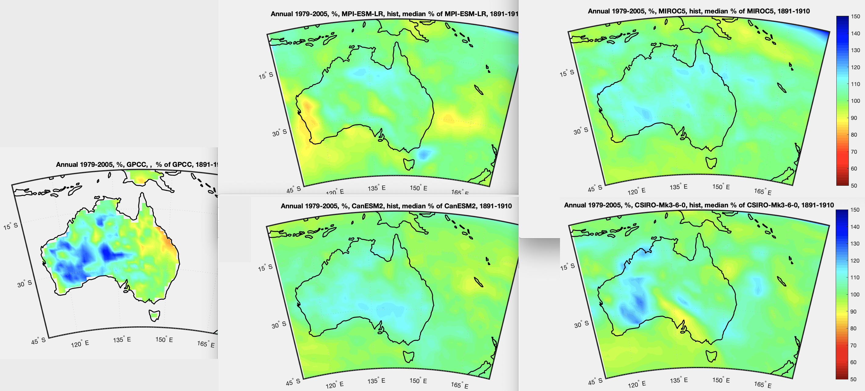
Figure 1 – Click to expand
So we are seeing how well the models compare among themselves, and with observations, for a century or so change. All of the models are run with the identical set of conditions (the best estimate of forcings like CO2, aerosols, etc) – that’s what CMIP5 is all about.
This second graphic is % comparison over Australian summer: December, January, February (DJF). It is otherwise exactly the same as the figure 1:
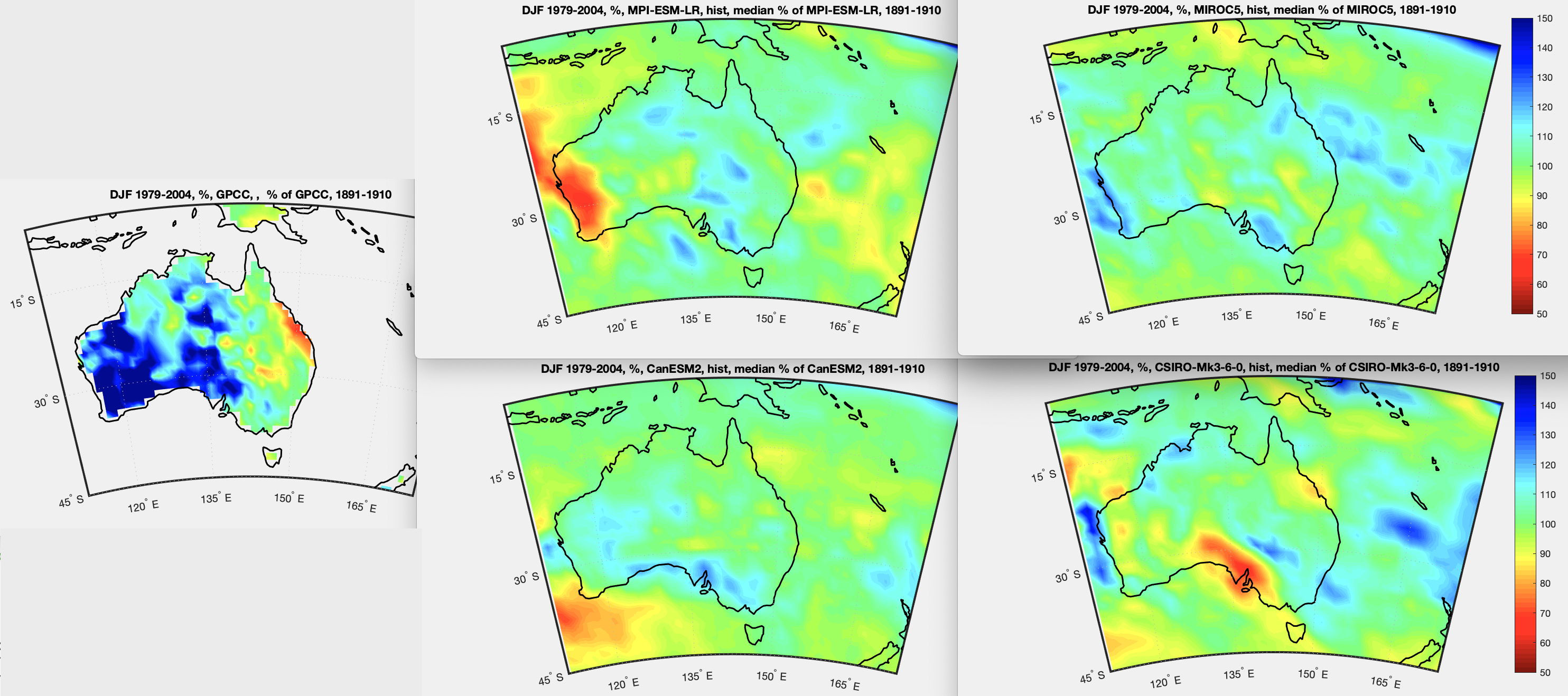
Figure 2 – Click to expand
The annual model comparisons look “better” than the summer (DJF) comparisons.
With the DJF comparisons, Australian summer observations across a century have the western half of Australia wetter, and coastal Queensland (that’s the right edge from halfway up) drier. Also some inland NSW regions drier.
MPI and CSIRO show the western edge drier. Miroc and CAN show the western edge wetter. CSIRO has the Adelaide region and west much drier, observations show much wetter, CAN and MPI show this area a little wetter while Miroc has it about the same.
It’s difficult to claim the summer model comparisons demonstrate any insight – given that we can check them against observations. And overall, these four models don’t demonstrate any particular biases, i.e., they don’t all agree with each other against the observations. Apart from inland western Australia where they fail to predict the much higher rainfall seen in observations.
Place yourself back in 1900. You have these models, how useful are they for predicting 100 years ahead what would happen to summer rainfall?
References
An overview of CMIP5 and the experiment design, Taylor, Stouffer & Meehl, AMS (2012)
GPCP data provided by the NOAA/OAR/ESRL PSL, Boulder, Colorado, USA, from their Web site at https://psl.noaa.gov/
GPCC data provided from https://psl.noaa.gov/data/gridded/data.gpcc.html
CMIP5 data provided by the portal at https://esgf-data.dkrz.de/search/cmip5-dkrz/
Notes
Note 1: The choice of dates is constrained by:
- 1891 being the start of the GPCC observational dataset
- 1979 being the start of the satellite era
- 2005 being the end date that this class of models ran to for their “historical” simulation – CMIP5 historical simulations were from 1850-2005
As a result, lots of comparisons in climate papers involve 1979-2005, so even though we aren’t using satellite data here, I have been using that 27-year period.
Note 2: Each model output is the median of all of the simulations


Australian winter, JJA, likewise compared:
Click to enlarge
[…] « Models and Rainfall – VI – Australia CanESM2, CSIRO, Miroc and MRI compared vs history […]
There’s something a bit odd about these graphs, seems to be suggesting that Western Australia was quite wet between 1979 and 2004… Especially in the Summer. I don’t think that is the case, certainly it’s not in the south of western Australia. It’s probably been the driest in recent history since the mid 70s. I don’t think there is any weather data in the interior of Western Australia )and possibly most of the state outside of the southwest corner for 1891 – 1910… So I wonder where GPCC got their numbers from
Nathan,
It’s a comparison with 1890-1910. Without digging in further, the actual area where most people people live (the coastal 100km) looks like “about no change” from the early period. For inland definitely looks like “lots more rain” compared with the early period.
I’ll see if I can dig into the actual totals, which will be very low.
GPCC is rain gauges.
Here’s a snapshot of rain gauge location from Global Precipitation Analysis Products of the GPCC, U Schnieder et al, 2015:
Click to enlarge
I doubt there were many rain gauges for that period in Western Australia outside of the southwest. I assume they have extrapolated?
Would it better to use a slightly more recent time frame, when the distribution is better?
As to the rain in the southwest, it’s clearly much less for the last 45 years or so (and apparently continuing to decline) – not only from rain data but also from stress on forests (old forests), much reduced stream flow (despite land clearing) etc.
Anyway just interesting they claim to have data, and that the it shows that in the southwest 1979-2004 was much the same.. Doesn’t align with my local understanding for the southwest.
http://www.bom.gov.au/climate/change/#tabs=Tracker&tracker=timeseries&tQ=graph%3Drain%26area%3Dswaus%26season%3D0112%26ave_yr%3D0
It’s interesting the difference in model results. Could it be the ‘wet models’ have more tropical cyclones; they would track down through the center where it is shown as wetter.
It actually is wetter in the Summer in the southwest compared to 1900-1910… But drier in an annual sense.
http://www.bom.gov.au/climate/change/#tabs=Tracker&tracker=timeseries&tQ=graph%3Drain%26area%3Dswaus%26season%3D1202%26ave_yr%3D0
http://www.bom.gov.au/climate/change/#tabs=Tracker&tracker=timeseries&tQ=graph%3Drain%26area%3Dswaus%26season%3D1202%26ave_yr%3D0
It was wetter in the Summer though…
Cliff Mass has a blog post that covers projected changes in rainfall (and temperature) using a high resolution (12 km) weather forecast model to refine the projections made by 12 different AOGCMs for the Pacific Northwest region.
https://cliffmass.blogspot.com/2020/10/what-will-northwest-weather-and-climate.html
The modeling starts in 1970 and Cliff’s graphs end in 2050 (though he apparently modeled out to 2100), so you can see 50 years worth of observed natural variability, in addition to a multi-model mean and interannual variability of each model and intermodal variability. Definitely worth the 10 minutes it takes to scan. Having both observed, hindcast and projected change and variability on the same graph gives me a much clearer understanding of the magnitude of both change and variability. To give readers a feeling for the quality information his figure convey, I’ll try to paste them below, (but may not succeed). The modeling is based on RCP8.5, but realistic scenarios don’t diverge much by then.
Seattle (KSEA) DJF Precipitation Observed and Modeled (1970-2050)


Seattle JJA Temperature Observed and Modeled (1970-2050)

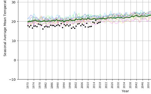
(Summer temps were systematically to warm and winter too cold).
Thanks Frank, very interesting data and article. The comments are also educational in their own way.
I see that the ensemble mean of the models fails to capture the inter-annual variability.
Even with the extreme scenario of RCP8.5 they project a little more rainfall for the region.
If anyone is confused, above there are duplicate copies of two graphs due to a mistake I made, one set for winter precipitation and one for summer temperature.
SOD correctly notes that the comments are interesting. Anytime a climate scientist has projections out to 2100, but only shows projections out to 2050, there will be questions and complaints. Apparently Cliff feels that the difference between emissions scenarios causes great uncertainty about the second half of the 21st century, but the differences between emissions scenarios by 2050 are small and RCP 8.5 is not an “extreme scenario” in 2050. He is also an optimist about the ability of technology to reduce emissions. Some of us will be around in 2050 to test these predictions.
I checked to see if there is a publication on this work and found a meeting presentation that was 10 minutes long. Very difference emphasis that blog post: “Are There Regional Climate Surprises That Can Only Be Determined by Dynamical Downscaling?” (The finds some).
https://ams.confex.com/ams/2020Annual/videogateway.cgi/id/516642?recordingid=516642