If you pay attention to the media reporting on “climate change” (note 1) you will often read/hear something like this:
Under a business as usual scenario..
And then some very worrying future outcomes. Less misleading, but still very misleading, you might read:
Under a high emissions scenario..
Every time I have checked the papers that are behind the press release faithfully reproduced by the stenographers in the media, they are referring to a model simulation using a scenario of CO2 emissions known as RCP8.5.
This scenario – explained below – is a fantastic scenario, and was not created because it was expected to happen.
So – calling it “business as usual”, charitably speaking, is from climate scientists who know nothing about history, demography, current & past trends. And uncharitably, is from climate scientists who are activists, pressing a cause, knowing that stenographers don’t do research or ask difficult questions.
I have been reading climate science for a long time – textbooks, papers, IPCC reports – and for sure when I read “under a business as usual scenario..” I always thought that climate scientists meant – “if we continue doing what we are doing, and don’t immediately reduce CO2 emissions”.
Then I read the papers on the scenarios.
—
Let me explain. It’s worth spending a few minutes of your time to understand this important subject..
Pre-industrial levels of CO2 were about 280ppm. Currently we are at just over 400ppm. Half a century ago climate scientists used rudimentary climate models and tried doubling CO2 to find out what the new climate equilibrium would be. Some time later people tried 3x and 4x the amount of CO2. It’s a good test. Do the simulated effects of CO2 on climate keep on increasing once we get past 2x CO2? Do the effects flat-line? Skyrocket?
Very worthwhile simulations.
Today we have lots of climate models. There are about 20 modeling centers around the world, each producing results that often vary significantly from other groups (more on that in future articles). How can we compare the results for 2100 from these different models? We need to know how much CO2 (and methane) will be emitted by human activity. We need to know land use and agricultural changes. Of course, no one knows what they will be, but for the purposes of comparison different modeling groups need to work from identical conditions (note 2).
So a bunch of scenarios were created, too many probably. It takes lots of computing power to run a simulation for 100 years. For IPCC AR5 in 2013 these were slimmed down to four Representative Concentration Pathways, or RCPs. One of these is RCP8.5.
The paper writers didn’t come up with RCP8.5 because they felt this was a likely scenario. They were told to come up with RCP8.5:
By design, the RCPs, as a set, cover the range of radiative forcing levels examined in the open literature and contain relevant information for climate model runs..
..The four RCPs together span the range of year 2100 radiative forcing values found in the open literature, i.e. from 2.6 to 8.5 W/m². The RCPs are the product of an innovative collaboration between integrated assessment modelers, climate modelers, terrestrial ecosystem modelers and emission inventory experts. The resulting product forms a comprehensive data set with high spatial and sectoral resolutions for the period extending to 2100..
..The RCPs are named according to radiative forcing target level for 2100. The radiative forcing estimates are based on the forcing of greenhouse gases and other forcing agents. The four selected RCPs were considered to be representative of the literature, and included one mitigation scenario leading to a very low forcing level (RCP2.6), two medium stabilization scenarios (RCP4.5/RCP6) and one very high baseline emission scenarios (RCP8.5).
From IPCC AR5, chapter 2, p.167 we can see that the change in CO2 per year (the bottom graph) is about 2ppm. The legend means, in English rather than maths, the increase in CO2 concentration in ppm per year:
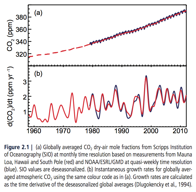
So a naive expectation based on current increases would be around 570 ppm in 2100 (410ppm + 80 years x 2ppm)
This is pretty close to the scenario RCP6, and a very long way from RCP8.5.
To get to RCP8.5 requires almost 1000ppm of CO2 (plus large increases in methane concentrations). This requires about 7ppm per year increase in CO2 starting soon. It’s a “fantastic” scenario that is extremely unlikely to happen, and if by some strange set of circumstances it was, the world could stop it simply by ensuring that sub-Saharan Africa had access to cheap natural gas, rather than coal (see note 3).
If climate scientists and media outlets wrote “under a very unlikely emissions scenario that we can’t see happening we get a few outlier models that predict..” it wouldn’t make good headlines.
It wouldn’t make good climate advocacy.
When you see a story about possible futures, check what scenario is being used. If it’s RCP8.5 (“business as usual” or “a high emissions scenario”) then you can just ignore it – or be concerned and start petitioning your government to encourage more natural gas production.
– Update Jan 1, 2019 (Dec 31st, 2018 in some parts of the world) -just added Opinions and Perspectives – 3.5 – Follow up to “How much CO2 will there be?” due to comments
Further Reading
Impacts – II – GHG Emissions Projections: SRES and RCP
Notes
Note 1: I put “climate change” in quotes to distinguish it from climate change that happened up until 1900 or thereabouts. I’m trying to keep this series non-technical, and also assume that readers haven’t read/remembered previous articles in the series. See Opinions and Perspectives – 2 – There is More than One Proposition in Climate Science
Note 2: A significant part of climate modeling is assessing results and trying to figure out why, say, the GISS model differs substantially from the MPI model. To do that we need to be sure that the model results are based on the same conditions.
Note 3: Natural gas produces about 1/2 the CO2 of coal, per unit of energy produced. If you read the paper for RCP8.5 you will see it depends upon a very high sub-Saharan African population burning huge amounts of coal. No demographic transition. No technological progress. A Victorian technology.


The rcp85 from 1861 to the present does not contain projections and assumptions about the future and serves as a frame of reference for comparing climate change theory with observational data. Pls see
https://tambonthongchai.com/2018/12/14/climateaction/
https://tambonthongchai.com/2018/09/25/a-test-for-ecs-climate-sensitivity-in-observational-data/
https://tambonthongchai.com/2018/09/08/climate-change-theory-vs-data/
https://tambonthongchai.com/2018/08/31/cmip5forcings/
Sincerely
Thongchai@fastmail.com
chaamjamal,
“..from 1861 to the present..”
And for the decade 2090-2100 does it contain assumptions about the future?
Yes sir
References for people interested, links found at Impacts – II – GHG Emissions Projections: SRES and RCP:
A special issue on the RCPs, Detlef P van Vuuren et al, Climatic Change (2011) – free paper
The representative concentration pathways: an overview, Detlef P van Vuuren et al, Climatic Change (2011) – free paper
RCP4.5: a pathway for stabilization of radiative forcing by 2100, Allison M. Thomson et al, Climatic Change (2011) – free paper
An emission pathway for stabilization at 6 Wm−2 radiative forcing, Toshihiko Masui et al, Climatic Change (2011) – free paper
RCP 8.5—A scenario of comparatively high greenhouse gas emissions, Keywan Riahi et al, Climatic Change (2011) – free paper
I have no where near the broad based education about climate that S.O.D. has, and offer this comment as a question to help my understanding.
When I used to teach a 101 level Physics of the Environment course I would teach about the benefits of replacing coal burning with methane burning, and the near doubling of output energy from burning methane carbon versus coal carbon. But this teaching on my part assumed that (A) the companies that are into this technology would work very hard to not leak the methane, since leak avoidance – at first glance – would get more energy to the customer per molecule of methane mined. But maybe (B) being really sloppy and careless, and leaking methane deliberately, helps the “bottom line” of those companies more than (A), because careful plumbing is more expensive than careless plumbing.
I was probably naive when I taught that course, because the assumption that scenario (A) would be preferred to the “routine leaking” scenario (B) ignored the rule IAATM; i.e. “Its ALL about the money”….
My subsequent reading about the techniques of the Koch Brothers in developing their fossle fuel industry, which involved the deliberate leaking of oil into water supplies, and about the measurements of leaking methane from methane energy producers, has lead me now to believe scenario (B) more than scenario (A). Hope I am wrong in now assuming that IAATM always wins out.
So maybe the “energy from methane” industry is doing more harm by deliberately leaking methane – a potent GHG, than the good they do by furnishing an alternative to coal and oil?
curiousdb, I don’t know what you read, but neither the Koch Brothers nor anyone else is deliberately leaking oil into water supplies.
At least he has now retired and no longer teaching young impressionable minds.
The climate modeling community has a >30 year history of calling implausible, exaggerated scenarios “business as usual,” for political purposes. That’s what James Hansen called his “Scenario A” when testifying to Congress, on June 23, 1988; here it is in the transcript:
http://sealevel.info/1988_Hansen_Senate_Testimony.html#scenariosABC
EXCERPT:
They considered the combined effects of five greenhouse gases: CO2, CFC11, CFC12, N2O, and CH4.
In their contemporaneous paper, they predicted a “warming of 0.5°C per decade” under “scenario A,” which they described as follows:
Now, I would agree that +0.5°C/decade would be something to worry about. Fortunately, it was nonsense.
Under their “scenario A,” emissions would have increased by 1.5% per year, totaling 47% in 26 years. In fact, CO2 emissions increased even faster than that. CO2 emissions increased by an average of 1.97% per year, totaling 66% in 26 years. Yet temperatures increased only about one-fourth as much as their “scenario A” prediction (or one-third according to GISTEMP).
Even so, climate alarmists frequently claim that the NASA GISS model was “remarkably accurate.” Only in the massively politicized field of climatology could a 200% to 300% error be described as remarkably accurate. Even economists are embarrassed by errors that large.
Additionally, the Hansen et al claim that an annual 1.5% (i.e., exponential) increase in GHGs causes an exponential “net greenhouse forcing” was a mindbogglingly obvious blunder. Even in 1988 it was common knowledge that CO2 (the most important of the GHGs they discussed) has a logarithmically diminishing effect on temperature. So an exponential increase in CO2 level causes a less-than-exponential increase in forcing (asymptotically approaching linear). Yet, apparently none of those eight illustrious authors recognized that that claim was wrong.
(BTW, note how linear the log(CO2), i.e., the “CO2 forcing,” has been for the last forty years.)
Additionally, their “Scenario B” description was self-contradictory. They wrote that it was for, “decreasing trace gas growth rates, such that the annual increase of the greenhouse climate forcing remains approximately constant at the present [1988] level.” But, of course, if GHG growth rates had decreased, then the annual increase of greenhouse forcing would have also decreased.
In fact, it wasn’t just their temperature projections which were wrong. Despite soaring CO2 emissions, even CO2 levels nevertheless rose more slowly than their “scenario A” prediction, because of the strong negative feedbacks which curbed CO2 level increases, a factor which Hansen et al did not anticipate. Although CO2 emissions increased by an average of 1.97%/year, CO2 levels increased by only about 0.501%/year (from 351.6 to 408.4 ppmv).
(Note: if that 0.501%/year exponential rate of CO2 increase continues for another 82 years, we’ll end the 21st century at 615 ppmv in year 2100, though the actual rate will probably decrease. To reach 1000 ppmv by 2100 would require annual CO2 increases averaging 1.11%, i.e., more than double the rate of the last 30 years.)
Additionally, including an exponential increase in CFCs in their “business as usual” Scenario A was indefensible, because the Montreal Protocol had already been agreed upon in 1987, and the Vienna Convention back in 1985. So there’s no excuse for Hansen’s August, 1988 paper nevertheless projecting exponential increases in CFCs, in any of their scenarios. That was not “business as usual,” it was “business as already outlawed.”
It is impossible to imagine that Hansen, his seven co-authors, the peer-reviewers, and the editors, were all ignorant of those already-existing treaties. They obviously knew CFC emissions would be falling, not rising. Yet they promoted a “scenario” as “business as usual,” which they knew was actually impossible.
In other words, although Hansen et al 1988 was wildly wrong about almost everything, it served its purpose. 5½ months after that testimony, and 3½ months after their paper was published, the United Nations created the Intergovernmental Panel on Climate Change, to combat the perceived global warming threat.
Only in the massively politicized field of climate change “skepticism” is such a misrepresentation considered acceptable. The Hansen projections are considered remarkably accurate after taking into account the actual GHG scenario which happened, which is between Scenario B and C.
The difference between scenarios was not primarily about CO2 – methane and CFCs (which were representing CFCs plus all other current and future man-made industrial gases) were the key differentiating factors. As it turned out, largely due to governmental mitigation policies (albeit primarily for non-climate change environmental issues) we followed lower concentration growth pathways for methane and CFCs.
This is similar to SoD’s error in the article above. The growth rate of CO2 has been steadily increasing over the past several decades. It was less than 0.2%/year 80 years ago, so assumption of a constant rate has no basis. And an assumption of a decline in the rate would require the opposite of historical reality.
The scenarios were created in 1983, so you assume knowledge of the future. And even at 1987, expected emission cuts in the original Montreal Protocol were so weak they were basically negligible. It was only with later modifications, mainly post-1990 that cuts were agreed which would halt CFC emissions. And, of course, non/minimal-Ozone depleting replacements for CFCs could be (and indeed were/are) GHGs as well.
I don’t know where you get these apologetics Paul as it seems wrong even when looking at Real Climate’s page on model comparisons to reality, Look at the regression rates of warming for GISS, and the scenarios. They are
“Scenarios from Hansen et al. (1988). Observations are the GISTEMP LOTI annual figures. Trends from 1984: GISTEMP: 0.19ºC/dec, Scenarios A, B, C: 0.33, 0.28, 0.17ºC respectively (all 95% CI ~±0.02). Last updated: 20 Jan 2018.”
Basically, reality is quite close to scenario C under which emissions were to cease in 2000.
This dodge about actual GHG concentrations is silly and misleading. Hansen made 2 errors that are big. 1. His GCM was primitive and too sensitive and 2. He dramatically overestimated emissions. These two errors both caused him to be badly wrong about the future in the alarming direction. It’s hard to explain these huge errors if everything was done in good faith.
dpy6629,
“Scenarios from Hansen et al. (1988). Observations are the GISTEMP LOTI annual figures. Trends from 1984: GISTEMP: 0.19ºC/dec, Scenarios A, B, C: 0.33, 0.28, 0.17ºC respectively (all 95% CI ~±0.02). Last updated: 20 Jan 2018.”
I get up to end of 2018: 0.33, 0.28, 0.15 and 0.19 in GISS, but yeah that seems about right. Not sure why you think that disagrees with what I said?
This dodge about actual GHG concentrations is silly and misleading.
It would be pointless to assess climate models against observations without considering the difference between scenarios.
1. His GCM was primitive and too sensitive and 2. He dramatically overestimated emissions.
I guess it’s obviously true that the GCM was primitive in comparison to current GCMs, how could it be otherwise? Too sensitive is still an open question. Probably so, but not definitive and many current models have similar sensitivity.
CO2 concentrations at 2018 are very close to Scenario A, and a bit higher than Scenario B. 2018 N2O concentrations are a bit lower than A and very close to B. Dramatically overestimated emissions is clearly not the case.
CFC concentrations were dramatically lower than Scenarios A and B, but bang on in Scenario C, which of course assumed the kind of strong mitigation which actually happened in the end. Methane concentrations were dramatically lower than in A and B after the plateauing in the 1990s, and close to Scenario C until the strong rise of the past several years. Since methane emission estimates are highly uncertain anyway it’s been difficult to quantitatively attribute this plateau, but it was clearly aided by policies against gas flaring, as well as policies against SO2 and CO emissions which would have affected the methane sink.
It’s hard to explain these huge errors if everything was done in good faith.
Not hard if one assesses in good faith.
Well OK Paul, so you seem to agree with my numbers and they indicate a quite high level of misoverestimation of how bad it would be. Trying to break it down in to several components and contending he might have been close on a single component is a form of apologetics and a distraction.
You seem to be just uncomfortable with how these results were described. That’s not worth arguing much about.
paulski wrote, “The growth rate of CO2 has been steadily increasing over the past several decades.”
The average CO2 growth rate calculated from 1988 (351.57 ppmv) to 2018 (about 408.4 ppmv) was +0.5007%/year.
The average CO2 growth rate calculated from 2008 (385.60 ppmv) to 2018 (about 408.4 ppmv) was +0.5761%/year.
So, yes, the growth rate increased, but only just barely.
paulski wrote, “The Hansen projections are considered remarkably accurate after taking into account the actual GHG scenario which happened, which is between Scenario B and C.”
That’s nonsense.
They described “Scenario C” as “draconian emission cuts… which would totally eliminate net trace gas growth by the year 2000.”
Obviously, nothing like that happened.
They described “Scenario B” as “decreasing trace gas growth rates.”
Obviously that didn’t happen, either, except for CFCs, which declined as required by the 1987 Montreal Protocol.
Hansen told Congress that “Scenario A” was “business as usual,” which means unless drastic public policy changes were made.
They had several different “Scenario A” warming rates in their paper, but all of them were way above reality (even if you use GISTEMP, the highest of all temperature indexes).
W/r/t GHGs other than CFCs, maybe it was just incompetence? Maybe. But it seems unlikely that all those illustrious authors could be that confused.
Could it really be true that they didn’t understand that “decreasing trace gas growth rates” would cause a decreasing annual increase of the greenhouse forcing? (They wrote that “decreasing trace gas growth rates” would cause an “approximately constant” annual increase in greenhouse forcing, which is obviously wrong.)
Could it really be true that they didn’t understand that rising CO2 levels cause a logarithmically diminishing increase in greenhouse forcing? (They wrote that an annual 1.5% [i.e., exponential] increase in GHGs would cause an exponential “net greenhouse forcing” increase, which is obviously wrong.)
But Hansen certainly knew that “Scenario A” was not “business as usual,” w/r/t CFCs.
If Michael Cohen deserves prison for lying to Congress, then James Hansen should be his cellmate.
What actually happened was roughly “business as usual,” except that subsequent revisions to the Montreal Protocol further reduced CFC emissions, even more than had been agreed to in 1988; however, the writing was already on the wall, even for that.
CO2 emissions increased even faster than the 1.5% Hansen et al projected, averaging nearly +2% per year. But CO2 levels were much less affected than they anticipated, since negative feedbacks removed over half of the added CO2 — which Hansen et al obviously did not expect.
Nobody really knows what CH4 emissions are, but CH4 levels rose in the first decade after 1988, plateaued in the second (nobody knows why!), and resumed rising in the third. Over thirty years, Mauna Loa CH4 level rose from 1.693 ppmv to 1.859 ppmv, an average annual increase of +0.3123%.
paulski wrote, “The growth rate of CO2 has been steadily increasing over the past several decades. It was less than 0.2%/year 80 years ago, so assumption of a constant rate has no basis.”
“No basis?” Take a look at this log-scale graph of CO2 level:
https://sealevel.info/co2_logscale_with_1960_highlighted.html
https://www.sealevel.info/co2.html?co2scale=2
Obviously the recent rate is much higher than the rate 80 years ago, but look how nearly straight that graph is for the last forty years. The CO2 forcing growth rate accelerated dramatically between about 1950 and about 1970, but only very slightly since then.
That straightening of the trace is the basis for assuming there will be no dramatic acceleration in CO2 forcing. We expect little or no acceleration in the future, because there has been little acceleration in CO2 forcing over the last forty years.
I wrote, “Additionally, including an exponential increase in CFCs in their “business as usual” Scenario A was indefensible, because the Montreal Protocol had already been agreed upon in 1987, and the Vienna Convention back in 1985”
paulski wrote, “The scenarios were created in 1983, so you assume knowledge of the future.”
Wrong. Hansen’s testimony was in mid-1988, and the paper was published two months later. 1988, not 1983. It didn’t take five years to run those simulations.
In 1988 Hansen told Congress that Scenario A represented “business as usual,” which was a plain lie. He knew perfectly well that CFCs would decline, rather than rise, because the treaty requiring that decline had already been ratified.
paulski wrote, “And even at 1987, expected emission cuts in the original Montreal Protocol were so weak they were basically negligible.”
This is from britanica.com:
That’s not “negligible,” that’s a very aggressive emission reduction schedule: -20% over five years, and -50% over ten. Yet Hansen’s “business as usual” scenario pretended that CFCs would increase, rather than decrease.
Come on, admit it: they were just plain dishonest.
dpy6629 wrote, “Hansen made 2 errors that are big. 1. His GCM was primitive and too sensitive and 2. He dramatically overestimated emissions.”
They also failed to anticipate that more than half of CO2 emissions would be removed from the atmosphere by negative climate feedbacks, like terrestrial greening, and ocean processes. Hansen et al basically assumed that emission growth and level increase are synonyms, which is very wrong. Mankind is adding the equivalent of about 5 ppmv of CO2 to the atmosphere each year, but CO2 levels are only rising by somewhere between 2 and 2.5 ppmv per year.
dpy6629 wrote, “Real Climate’s page on model comparisons to reality… Scenarios A, B, C: 0.33, 0.28, 0.17ºC respectively.”
Hansen et al 1988 is inconsistent in the amount of warming which it predicts for Scenario A. On p.9346 they wrote, “The 1ºC level of warming is exceeded during the next few decades in both scenarios A and B; in scenario A that level of warming is reached in less than 20 years.”
Likewise, on p. 9357 they wrote, “We also conclude that if the world follows a course between scenarios A and B, the temperature changes within several decades will become large enough to have major effects on the quality of life for mankind in many regions.
The computed temperature changes are sufficient to have a large impact on other parts of the biosphere. A warming of 0.5ºC per decade implies typically a poleward shift of isotherms by 50 to 75 km per decade…”
However, their Fig. 3a shows a Scenario A warming rate of only about 0.36 ºC / decade for 1988 [then current] to 2019.
OTOH, their Fig. 3b shows a Scenario A warming rate which accelerates to about 0.75 ºC / decade for the period 2040-2060.
daveburton,
They described “Scenario C” as “draconian emission cuts… which would totally eliminate net trace gas growth by the year 2000.”
Obviously, nothing like that happened.
Yes, it did. CFCs were subject to draconian emission cuts, as were carbon monoxide and SO2.
They described “Scenario B” as “decreasing trace gas growth rates.”
Obviously that didn’t happen…
Yes, it did. Methane substantially decreased in growth rate.
Seriously, all the numbers are available from the original work. This is very easy stuff to check without relying on your subjective interpretation of wording.
Hansen told Congress that “Scenario A” was “business as usual,” which means unless drastic public policy changes were made.
And drastic public policy changes were made. Just not with regards CO2, which of course has tracked closely with Scenario A.
W/r/t GHGs other than CFCs, maybe it was just incompetence? Maybe. But it seems unlikely that all those illustrious authors could be that confused.
They weren’t confused or incompetent. The scenarios used were entirely reasonable and valid at the time.
Could it really be true that they didn’t understand that “decreasing trace gas growth rates”…
You’re getting pointlessly hung up on words again. All the numbers are available, there’s no need for this self-imposed obfuscation.
“No basis?” Take a look at this log-scale graph of CO2 level
Interesting sleight of hand there, changing from CO2 growth rates to log CO2 growth rates. Over the full Mauna Loa record the percentage CO2 growth rate has increased from a little under 0.3%/year to over 0.6%/year. Taking the best fit linear regression of percentage growth rate through the full record and extrapolating to 2100 the growth rate at the end of the Century is 1.1% and concentration is 828ppm. Even applying the regression only to your cherry-picked 40-year period 2100 concentration is 794ppm and reaches the RCP8.5 level of 935ppm in 2116. A whopping 16 year delay.
Wrong. Hansen’s testimony was in mid-1988, and the paper was published two months later. 1988, not 1983.
Wow, that’s ignorant. You believe he just knocked up the model simulations in a free afternoon? From the paper:
paulski0 wrote, “CFCs were subject to draconian emission cuts, as were carbon monoxide and SO2.”
Carbon monoxide and SO2 are not greenhouse gases.
They were already declining, too. In fact, the decline in sulfur emissions (in part because of worries over acid rain), and consequent decline in sulfate aerosols in the atmosphere, contributed to the sharp warming in the 1980s and early 1990s. (SO2 does absorb around 7.4 µm, which is in the short-wavelength tail of the Earth’s emission spectrum, but the Earth’s emissions there are mostly from warm places, which are also mostly humid places, and water vapor also absorbs heavily there. So, practically speaking, SO2 is not a GHG.)
I wrote, “Take a look at this log-scale graph of CO2 level…”
paulski0 replied, “Interesting sleight of hand there, changing from CO2 growth rates to log CO2 growth rates.”
That’s not “slight of hand.” Do you not understand that CO2’s “greenhouse forcing” is logarithmically diminishing? A log-scale graph of CO2 level is a graph of its effect on temperatures.
That’s not “slight of hand,” that’s clarification.
paulski0 replied, “Over the full Mauna Loa record the percentage CO2 growth rate has increased from a little under 0.3%/year to over 0.6%/year.”
Now that is slight of hand. I just showed you the graph where you can see that most of the acceleration occurred in the early years.
Mauna Loa measurements began in 1958. Here are the decadal rates of increase in CO2 level (from here):
1958 315.34 ppmv (strong El Nino)
+0.2415 %/yr (average increase, 1958-1968)
1968 323.04 ppmv (moderate El Nino)
+0.3762 %/yr
1978 335.40 ppmv (ENSO neutral)
+0.4720 %/yr
1988 351.57 ppmv (moderate El Nino)
+0.4222 %/yr
1998 366.70 ppmv (very strong El Nino)
+0.5038 %/yr
2008 385.60 ppmv (weak La Nina)
+0.5761 %/yr (average increase, 2008-2018)
2018 ≈408.4 ppmv (ENSO neutral)
So, yes, from 1958 to 1968 the CO2 level increased an average of only 0.24% per year. But from 1968 to 1978 the CO2 level increased an average of 0.37% per year, and from 1978 to 1988 it increased 0.47% per year.
Since then it’s increased only a little (and it actually has not gotten to “over 0.6%/year,” so far).
paulski0 wrote, “You’re getting pointlessly hung up on words again.”
I pointed out that some of what Hansen & his seven illustrious co-authors wrote in that paper was very obviously untrue.
When I say “obviously” I mean obvious even then, not just in retrospect.
That’s not being “pointlessly hung up on words again.”
They wrote that “decreasing trace gas growth rates” would cause an “approximately constant” annual increase in greenhouse forcing. They also wrote that an annual 1.5% [i.e., exponential] increase in GHGs would cause an exponential “net greenhouse forcing” increase. Both of those statements are so obviously wrong that I cannot imagine how that paper got through peer-review containing such errors.
paulski0, wrote, “Wow, that’s ignorant. You believe he just knocked up the model simulations in a free afternoon?”
Ignorant or not, at least I do know that CO and SO2 are not GHGs.
I also know that it didn’t take months for a single run of their simulation. They made many, many runs, while debugging their Fortran code.
51 weeks elapsed between the signing of the Montreal Protocol and the publication of Hansen et al 1988. They had plenty of time to plug in realistic values for CFCs and re-run their simulations. They simply chose not to.
If they had done so, then their projections wouldn’t have been so scary. They were trying to frighten the politicians into supporting creation of the IPCC, so the projections had to be as frightening as possible.
PaulS, With respect I’m seeing a lot dodging and weaving here.
You say concerning Scenario C that indeed CFC’s, CO, and SO2 were subjected to cuts. In the case of SO2 however, clearly not “draconian” cuts. Of course, CO2 and methane continued to grow about as fast as before. SO2 is a negative forcing as you know. So total forcing continued to grow rather rapidly. Reality turned out to be quite inconsistent with Scenario C.
if Hansen had total forcings for his scenarios I’d be interest in them. I’d wager that total GHG forcing is somewhere close to scenario B and a lot higher than Scenario C. In any case, “effective forcing” is different in different models so that perhaps makes it impossible to accurately evaluate this accurately.
Bottom line: Hansen’s plot and his verbal descriptions (which may or may not match the internal numbers you cite) were in my estimation designed to scare people by showing that things could get quite bad in just 20 years unless we went with scenario C with “draconian emission cuts”. Reality was not nearly as scary and we didn’t do the majority of those emissions cuts.
Current GISS climate model I think has an ECS of 2.3C. I recall that Hansen’s model in 1988 had an ECS north of 4C. That’s a significance difference.
There have been a number of blog posts attempting to determine how well Hansen’s projections have turned out. (Moyhu had a decent summary in 2016). I personally haven’t been convinced by any of them.
The projected forcing change in all of Hansen’s scenarios was far off. Scenario A ignored the agreed upon, but unsigned terms of Montreal Protocol and assumed massive increases in CFC. CH4 was too high; CO2 modestly low. He put two volcanic eruptions (one still in the future) in Scenario B and plateaued CO2 emissions in 2005 in Scenario C. If the scientific method is to devise a hypothesis about how the world behaves (a climate model is a hypothesis), Hansen did a lousy job of making a testable prediction that could be used to invalidate his hypothesis. (AOGCMs are used by the climate science community to influence policy, not practice the scientific method.)
What we really want to know is the TCR associated with Hansen’s projections and compare with TCR observed over the same period. One difficult problem is deciding on the temperature at appropriate starting point, ie T(t=0). There was a large El Nino event in 82/83 right at the beginning of Hansen’s projection period. The best way to determine deltaT is to do a least-squares fit to the temperature data and multiply the trend by the period. That way, T(t=0), the y-intercept on a plot, and deltaT are being determined by all of the data, not a arbitrary choice. Most bloggers show an overlay where the y-intercept is chosen by eyeball. (Insanity.)
Another big problem is that “committed warming” and the recovery period after a large volcanic eruption depend on ECS as well as TCR. Hansen’s model (IIRC) had an ECS of 4 K, and therefore takes a long time for the effect of large eruptions to stop perturbing estimates of TCR. When working with energy balance models, Nic Lewis chooses baseline periods as far from eruptions as possible and averages over a 20-year period to eliminate the effects of ENSO and other forms of unforced variability. This leaves Scenario A as the only useful projection, albeit with one with too much forcing.
So a complete analysis is really complicated. A simpler answer: From Otto (2013), written by IPCC royalty, we know that TCR for the 1970-2009 period was 1.4 K (0.7-2.5 90% ci) and 1.3 K (0.9-2.0 K) for the best defined sub-period. I suspect the last decade hasn’t changed this too much (and would blame the 15/16 El Nino if it has.) With an ECS of 4.0, the only way Hansen’s model could have exhibited a TCR reasonably consistent with Otto (2013) is for its ocean heat uptake, deltaQ, to be unrealistically high and disagree with ARGO.
TCR = F2x*(dT/dF)
ECS = F2x*(dT/(dF-dQ))
TCR/ECS = (dF-dQ)/dF = 1 – dQ/dF
So I’m confident (perhaps over-confident) that Hansen’s model must be inconsistent with observations OR appears consistent with observations only because the warming expected given its high ECS has been suppressed by sending too much heat into the deep ocean. The consensus is busy trying to explain why energy balance models disagree with AOGCMs, which means they think this disagreement is real. Otto (2013) studied observed warming and forcing in the period relevant to judging whether Hansen’s projections were correct. They acknowledged an apparent disagreement between the central estimates of AOGCMs and EBMs. Anyone who believes this dilemma somehow magically doesn’t apply to Hansen’s 1988 AOGCM is probably being fooled by some of the complications mentioned above.
This is very wrong. RCP8.5 is a business-as-usual scenario according to the actual definition of “business-as-usual”, which is a scenario without any policy attempts to mitigate against climate change. The term has now largely been replaced by “baseline” or “reference” in scenario and IPCC literature, but BaU persists in wider literature due to being better known as a term.
It is often used as the business-as-usual scenario simply because it is actually the only BaU/baseline/reference scenario in the RCPs – all the others assume some amount of mitigation policy. There are of course other possible BaUs, and RCP7 is due to be introduced for CMIP6/AR6 as another BaU/baseline pathway.
This is very misleading. The same is equally true for all RCPs
That’s absurd. 80 years ago CO2 was rising at about 0.4ppm/year. The average rise in the past several years has been about 2.5ppm/year. Equivalent growth over the next 80 years would see CO2 rises of over 15ppm/year by 2100.
You’ve presented no evidence at all to support that belief.
And that’s not at all “fantastic”? Is there even enough natural gas to satisfy that level of future demand?
Sounds like stealth activism to me.
Paulski0: Some information on RCP8.5 from the paper that defined it:
https://link.springer.com/article/10.1007%2Fs10584-011-0149-y
“The [RCP8.5] scenario’s storyline describes a heterogeneous world with continuously increasing global population, resulting in a global population of 12 billion by 2100. Per capita income growth is slow and both internationally as well as regionally there is only little convergence between high and low income countries. Global GDP reaches around 250 trillion US2005$ in 2100. The slow economic development also implies little progress in terms of efficiency. Combined with the high population growth, this leads to high energy demands. Still, international trade in energy and technology is limited and overall rates of technological progress is modest. The inherent emphasis on greater self-sufficiency of individual countries and regions assumed in the scenario implies a reliance on domestically available resources. Resource availability is not necessarily a constraint but easily accessible conventional oil and gas become relatively scarce in comparison to more difficult to harvest unconventional fuels like tar sands or oil shale. Given the overall slow rate of technological improvements in low-carbon technologies, the future energy system moves toward coal-intensive technology choices with high GHG emissions. Environmental concerns in the A2 world are locally strong, especially in high and medium income regions. Food security is also a major concern, especially in low-income regions and agricultural productivity increases to feed a steadily increasing population.8
Compared to the broader integrated assessment literature, the RCP8.5 represents thus a scenario with high global population and intermediate development in terms of total GDP (Fig. 4). Per capita income, however, stays at comparatively low levels of about 20,000 US$2005 in the long term (2100), which is considerably below the median of the scenario literature. Another important characteristic of the RCP8.5 scenario is its relatively slow improvement in primary energy intensity of 0.5% per year over the course of the century. This trend reflects the storyline assumption of slow technological change. Energy intensity improvement rates are thus well below historical average (about 1% per year between 1940 and 2000). Compared to the scenario literature RCP8.5 depicts thus a relatively conservative business as usual case with low income, high population and high energy demand due to only modest improvements in energy intensity (Fig. 4).”
“Coal use in particular increases almost 10 fold by 2100 and there is a continued reliance on oil in the transportation sector.”
IMO, 12 billion people in 2100 and 0.5%/yr improvement in energy intensity (less than half of the historic rate) can hardly be considered “business-as-usual”.
If you read the RCP6.0 scenario, it assumes that radiative forcing would rise to 7.0 W/m2 without any restrictions following the B2 development scenario and then adds emissions reductions after 2050 to reach a plateau at 6.0 W/m2. (GDP increases 7.5X or 2%/yr from 2000 to 2100 and population to 9.8 billion.) You say that an RCP7.0 pathway will be added for AR6. That looks more like a business-as-usual scenario.
You wrote: “80 years ago CO2 was rising at about 0.4ppm/year. The average rise in the past several years has been about 2.5ppm/year. Equivalent growth over the next 80 years would see CO2 rises of over 15ppm/year by 2100.”
RCP 8.5 has CO2 reaching over 900 ppm, an average annual growth rate of of 6.2 ppm/yr over 80 years and more than 10 ppm/yr in 2100 by linear extrapolation. However, the per capita emission rate in the developed world plateaued long ago, so future emission growth will occur in the developing world they should also approach a plateau. China’s per capital emissions are already the same as the EU and they are promising to reach a plateau in a decade even though they have high dependence on coal right now. The idea that CO2 will someday be rising 10 ppm comes from the assumption that we will be burning 10-fold more coal than we do today. Even that assumption is 50% short of your 15 ppm/yr extrapolation for 2100. RCP 6.0 puts us at about 650 ppm in 2100 and a business as usual RCP7.0 might be 700 ppm. Those represent average growth rates of 3-4 ppm/yr over 80 years.
IMO, 12 billion people in 2100 and 0.5%/yr improvement in energy intensity (less than half of the historic rate) can hardly be considered “business-as-usual”.
And on what basis are you making that judgement with regards population? I mean, world population was at about 2 billion 80 years ago. Why couldn’t it increase by another 5 billion over the next 80 years? Of course, the reality of population demographics is more complex than that, which analogously I’ve tried to point out with regards the absurd 2ppm/year extrapolations. 12 billion is above the current median UN demographic projection, but not by a lot, and well within uncertainties.
In any case the new RCP8.5-equivalent (SSP5) has 2100 population of 7 billion and it looks like average energy intensity improvement of greater than 1%/year, so these points are not very relevant for the plausibility of RCP8.5.
You say that an RCP7.0 pathway will be added for AR6. That looks more like a business-as-usual scenario.
If you mean that RCP7 is a more likely (even much more likely) business-as-usual/baseline scenario than RCP8.5 then I would agree, as far as we can see right now. That’s pretty close to the median of the range of baseline scenarios, which is about as good as it gets for assessing probabilities of these things.
China’s per capital emissions are already the same as the EU and they are promising to reach a plateau in a decade even though they have high dependence on coal right now. The idea that CO2 will someday be rising 10 ppm comes from the assumption that we will be burning 10-fold more coal than we do today. Even that assumption is 50% short of your 15 ppm/yr extrapolation for 2100.
Not really sure what your point is here. My extrapolation was to point out that CO2 has not simply been rising by 2ppm/year forever – it has grown – and therefore extrapolating 2ppm/year is ridiculous. If you take into account the growth rate in CO2 increase over the past 100 years, then clearly rates of 15ppm/year are plausible by 2100 if the growth rate continues as it has historically.
Yes, we would have to increase coal consumption by a lot. I believe tenfold is an overestimate in comparison to today, an overestimate I’ve seen bandied about before. It comes partly from using year 2000 as “today” when coal consumption today is about 60-70% greater than it was then. And also from rounding up to 10 from about 8-9 in comparison to year 2000. Again, nothing we haven’t seen from past growth. How many people in 1900 would have believed that global coal consumption in 2018 would have increased nearly tenfold? I suspect there would be many who would be disbelieving.
But the other thing is that China’s promise is one specifically concerning climate change mitigation, which means it isn’t relevant for assessing inherent plausibility of baseline no-mitigation scenarios. Obviously RCP8.5 isn’t going to happen if we enact mitigation policies.
Paulski wrote:
“And on what basis are you making that judgement with regards population? I mean, world population was at about 2 billion 80 years ago. Why couldn’t it increase by another 5 billion over the next 80 years?”
There are a range of logical projections for population growth and a single value for a central estimated that belongs in a “business-as-usual” scenario. By raising that projection to 12 billion people in 2100, RCP8.5 is on its way to becoming a “worst case” scenario.
Projected emissions are a function of projected: population times GDP/capita times energy consumption/GDP times CO2/energy consumption. The last factor is energy intensity, which RCP8.5 assumed is going to improve at half of the 1940-2000 rate, despite the efforts that are and will be made. Is this a business-as-usual scenario or a worst-case scenario?
SOD asserted that RCP8.5 shouldn’t be characterized as a business-as-usual scenario. Isn’t he right? Isn’t the appropriate question now whether an RCP7.0 scenario can be characterized as “business-as-usual”?
Paulski wrote: If you take into account the growth rate in CO2 increase over the past 100 years, then clearly rates of 15ppm/year are plausible by 2100 if the growth rate continues as it has historically.
But not plausible if you apply the Kaya identity and examine each of the factors that contribute to the growth of CO2 emissions. As I pointed out, RCP6.0 and 7.0 project CO2 rising an average of 3-4 ppm/yr, far closer to SOD’s underestimate of 2.0 ppm/yr than your 15 ppm/yr.
Well if its Business as Usual, it shows incredible ignorance of the energy industry. Gradually, coal is being displaced by natural gas and in the US its mostly already happened.
Natural gas is cleaner and cheaper than coal and a lot safer to produce. There are huge differences in sulphur emissions (which are going to be mitigated as countries worry more about air pollution). Natural gas has low sulphur content. Then there is fly ash and particulates, which also need to be mitigated with coal.
It seems quite likely that simple economics and people’s desire for clean air and water will lead to the phase out of coal over the next few decades. There may be exceptions due to Green fanaticism such as in Germany’s phaseout of nuclear power, but most countries are not that crazy.
On this basis alone, RCP 8.5 is a “worst case” scenario that is extremely unlikely to happen. SOD is exactly right about that.
dpy6629,
The previous generation of scenarios were developed a decade or so ago, so wouldn’t have had much visibility of changes in natural gas. The new SSP5 scenario does appear to feature much more natural gas supply than the old scenario used for RCP8.5 emissions. Coal consumption appears to plateau between 2010 and 2030 before growing again as natural gas extraction fails to keep up with demand:
From the New York Times (Oct. 9, 2009)
“Because so little drilling has been done in shale fields outside of the United States and Canada, gas analysts have made a wide array of estimates for how much shale gas could be tapped globally. Even the most conservative estimates are enormous, projecting at least a 20 percent increase in the world’s known reserves of natural gas.
One recent study by IHS Cambridge Energy Research Associates, a consulting group, calculated that the recoverable shale gas outside of North America could turn out to be equivalent to 211 years’ worth of natural gas consumption in the United States at the present level of demand, and maybe as much as 690 years. The low figure would represent a 50 percent increase in the world’s known gas reserves, and the high figure, a 160 percent increase.”
It is also true that generally the history here is that official estimates have underestimated recoverable reserves. Given the superiority of natural gas over coal economically and environmentally, it seems likely that coal will be increasingly phased out even by developing countries.
dpy6629,
If we take the central estimates there it says that these sources could possibly double global natural gas reserves, and that would be enough to supply current United States usage for about 800 years.
So, what does that mean globally and for the future? US consumption of natural gas is about 20% of global, so that’s 160 years at current usage rates. Entirely replacing coal at current energy demand would require greater than a doubling of natural gas consumption, so we’re down to less than 80 years. And demand is likely to roughly double over the next 30 years (meaning quadruple current natural gas consumption). I could work it out with a spreadsheet, but you can see it’s basically all gone by about 2070.
Presumably there will be further discoveries in future which will extend reserves, but it looks pretty likely natural gas production will stop growing from mid-century.
In any case, natural gas is still a fossil fuel even if it’s a better one than coal. All you do by transitioning from coal to gas is delay RCP8.5 by a couple of decades.
OK Paul, assuming your arithmetic is correct, that’s still 50 years of clean natural gas and pretty large benefits. It is also true that much of the world has not really been evaluated carefully for shale gas so that there is likely much more out there.
The problem I have with all these scary stories is that they usually assume little new technology or adaptation. In reality technological innovation has been accelerating for at least a century. Human beings are quite creative and human society good at adapting to new challenges. That’s why SOD I think is correct about RCP 8.5.
The track record for these worst case scenarios is really bad. There have been literally scores of these scary scenarios from Ehrlich and the population bomb to the AIDS will spread like wildfire to the entire population. You perhaps remember the copper shortage scare from around 2000. Usually these scary stories are public relations spin from special interest looking for more money to “solve” the problem or fund their research.
I think daveburton comes very close to CO2 increase when he writes: “Note: if that 0.501%/year exponential rate of CO2 increase continues for another 82 years, we’ll end the 21st century at 615 ppmv in year 2100”
CO2 measurements from 1958 until now, do show an increse of about 0,5% pr year. (systematic measures began in 1958)
This is result of business as usual: 0,5 % pr year. An it is remarkable steady.
If we follow Hansen and say that “business as usual” gives CO2 emission increased of 1,5% pr year (scenario A), and that this results in 0,5% more CO2 in the air (as shown), we will still have plenty of time to se how it develops without rushing to solutions.
And I think I will disagree with myself here. The growth in CO2 emission is more of a linear growth than an exponential growth. From 1958 to 2017 it has increased from about 8000 million tons to about 37000 million tons. 480 million tons increase pr year. And this linear growth results in an exponential growth of CO2 in the air, an increase of 0,5% pr year.
This is what I will call “business as usual”.
Methane and nitrous oxide also show a small linear growth over the last 50 years.
The experts have spoken.
The United Nations Environment Programme (UNEP, 2011) looked at how world emissions might develop out to the year 2020 depending on different policy decisions. To produce their report, UNEP (2011)[ convened 55 scientists and experts from 28 scientific groups across 15 countries.
“Projections, assuming no new efforts to reduce emissions or based on the “business-as-usual” hypothetical trend, suggested global emissions in 2020 of 56 gigatonnes CO2 equivalent (GtCO2-eq), with a range of 55-59 GtCO2″
So how could all these scientists be so wrong about “business-as-usual”
There will be emission of about 40 gigatonnes CO2 in 2020. And little has really changed these 7 years. Emission has only moved from US and Europe to China, India and some other “developing countries”. So world business is as usual.
Strange to se that it is so easy to deceive 55 scientists and experts with a business as usual scenario.
nobodysknowledge wrote, “out to the year 2020… 56 gigatonnes CO2 equivalent… 40 gigatonnes CO2 in 2020…”
The former figure includes other GHGs, the later just CO2, itself.
daveburton. Correction received. Thank you.
Methan 8000 million tons CO2 eqv in 2012, increasing 100 mill ton pr year, gives 8800 million tons in 2020. Nitrous oxide 3150 million tons CO2 eqv in 2012, increasing 30 mill tons pr year, gives 3400 million tons in 2020. CO2 35500 million tons in 2012, increasing 480 million tons pr year, gives 39100 million tons in 2020.
Right answer is CO2 equvalent emission 2020: 51300 million tons CO2 eqv.
Still “scientists and experts” are far out.
In 2012 the projections of business as usual were even higher than the year before: ”
The report, which involved 55 scientists from more than 20 countries, said the projected 2020 emissions of 58Gt that would result from business as usual leave a gap bigger than projected in the 2010 and 2011 UNEP assessments. This expansion is in part a result of projected economic growth in key developing economies and a phenomenon known as ‘double counting’ of emission offsets.
The Emissions Gap Report 2012 points out that even if the most ambitious level of pledges and commitments were implemented by all countries – and under the strictest set of rules – there would be a gap of 8 Gt of CO2 equivalent by 2020. This is 2 Gt higher than last year’s assessment.”
It looks like the values are 15% higher in the business as usual scenario compared with emissions from consumption, production and transport. This includes forestry fires, forestry wood decay, forestry drained peat decay and peat fires, and waste.
This is not true. As with other RCPs, some scenarios have high population growth, some low population growth. The scenario used to represent RCP8.5 for CMIP5 modelling had relatively high population growth, though well within demographic projections. The RCP8.5-equivalent A1FI from SRES had low population growth, as does the new RCP8.5-equivalent which came from the SSPs. 2100 population about 7 billion.
Perhaps you’re unware that, with all the technological progress over the past 100+ years, we actually burn almost 10 times as much coal as we did at the end of the Victorian era.
Paulski: If you accept the figures in this Wikipedia article, the only places left in the world with high fertility rates (3-8 children/woman are in sub-Saharan Africa (except South Africa) and Afghanistan. The greatest uncertainty presumably lies in the rate at which the fertility rate in these remaining fast-growing areas drops. RCP6.0 calls for 10 billion people by the end of the century and RCP8.5 12 billion. Some estimates for 2100 are as low as 8 billion.
https://en.wikipedia.org/wiki/Projections_of_population_growth
Frank,
I didn’t suggest that sub-Saharan Africa isn’t the greatest source of uncertainty with regards future population growth. What I pointed out is that high population growth is not at all required for RCP8.5 level forcing. A1FI and SSP5 are both RCP8.5 level scenarios with 2100 population at only 7 billion.
Paulski: I’ve heard A1F1 referred as a golden age where all nations become fully developed, but are dependent on coal for the vast majority of their energy. In other words, amazing progress on everything – but low-carbon energy. However, I don’t want to look up the details of two more scenarios and debate the merits of describing either one business-as-usual after there is already a good case that the scenario published for RCP8.5 is IMO not business-as-usual.
It seems to me that RCP6.0 made some reasonable assumptions (that might be characterized as business-as-usual) and arranged for forcing to reach a plateau by 2100 (IIRC by applying a carbon tax beginning in 2050). So I’m happy to say business-as-usual is somewhere between RCP6.0 and 8.5.
Hi Dave Burton, above:
From Reuters, Sept 29, 2000
from “U.S.Indicts Koch Brothers on Pollution Violations in Texas”
“Early this year, Koch agreed to pay a $30 million civil fine for violating the Clean Water Act; the fine was the largest ever imposed on a company for violating the law. It also settled suits that accused it of spilling millions of gallons of oil from its pipelines into waters and wetlands in six states. The $35 million settlement resolved suits by the federal government and Texas regarding spills in Alabama, Kansas, Louisiana, Missouri, Oklahoma and Texas.”
The principle is that fossil energy is so cheap to the producers that they can waste a lot of energy by using bad plumbing and increase their profits thereby. Slip shod plumbing is enough cheaper than careful plumbing to warrent polluting water supplies for increased profits. In a later post I will discuss methane production in this light.
curiousdp,
A good example of activist propaganda:
“Scientists Yangyang Xu and Veerabhadran Ramanathan found in a paper published in the Proceedings of the National Academy of Sciences (PNAS) that there already exists a 1 in 20 chance that the 2.2 trillion tons of carbon dioxide in the Earth’s atmosphere could cause an existential warming threat. This “fat tail” scenario would mean the world experiences “existential/unknown” warming by 2100 — defined in the report as more than 5 degrees Celsius above preindustrial levels.
Temperatures haven’t been that high since the Miocene warming period. That low-probability but very extreme scenario could expose most of the world’s people to deadly heat stress, with 2.5 billion facing viruses linked to warming and 20 percent of the world’s species becoming extinct.
“To put in perspective, how many of us would choose to buckle our grandchildren to an airplane seat if we knew there was as much as a 1 in 20 chance of the plane crashing?” said Ramanathan in a statement. “With climate change that can pose existential threats, we have already put them in that plane.”
The report also found a 50 percent chance that temperatures would rise to 4 C under a business-as-usual scenario, a less extreme but still highly dangerous level. The long-term goal of the Paris accord was to maintain warming well below 2 C.”
https://www.scientificamerican.com/article/the-window-is-closing-to-avoid-dangerous-global-warming/
First the catastrophe and then the highly dangerous business-as-usual. Without saying anything about what is usual.
So I think that it is very clear that the term “business-as-usual” is used in a rhetoric of propaganda.
And if you succed in dehumanizing your opponent. “He will put our children in a crashing plane”. Then it is a rhetoric of war.
Hello,
I heard that the first CO2 emitter/absorber are the oceans, far ahead this patsy subsaharian people and also the chineses coal central (rcp 8.5 takes care of the dimming effect, right ?).
Did these models having all data about the capacity of the oceans to absob the same quantity of CO2 (acidification) to maintain the actual rate or will a saturation come, because heat/surface temperature decrease the dissolving, and may skyrockets this rate ?
There’s no danger that the oceans will become saturated with CO2.
To start with, the oceans contain about 50× as much CO2 as the atmosphere. So it’s hard to affect the whole ocean very much, with atmospheric CO2 emissions. However, the ocean mixes very slowly, so you could still get an effect on surface waters.
AR5 estimate [Fig 6.1] that the oceans current remove about 26% of the CO2 that mankind emits into the atmosphere:

Note: the units shown in that illustration are PgC (“petagrams carbon”). To convert those numbers to more familiar Gt CO2, multiply them by 3.667 Gt CO2 / PgC:
2.3 ±0.7 PgC = 8.4 ±2.6 Gt CO2 added to the oceans, per year.
To convert that to its equivalent in atmospheric CO2, divide by 8.053 Gt CO2 / ppmv CO2 = 0.7 to 1.4 ppmv of atmospheric CO2.
That atmosphere retains about twice that much.
However, not all the CO2 dissolved into the upper layer of the ocean stays there. Some if it obviously mixes with deep water, but that’s a very slow process. Additionally, biological processes tend to convert it to calcium carbonate shells, which drift downward into the ocean depths.
Some of that sequestered carbon settles on the ocean floor, but I’ve read that most of it probably redissolves into the water, on the way down, under the high pressures of the ocean depths, though I don’t recall seeing any quantitative estimates.
Anyhow, the higher CO2 levels go, the faster the oceans will remove it from the atmosphere. That’s one of the important negative feedback mechanisms which work to stabilize atmospheric CO2 levels, and reduce the effect of anthropogenic CO2 emissions.
s/ AR5 estimate [Fig 6.1] that the oceans current remove/ AR5 estimates [Fig 6.1] that the oceans currently remove/
I seem to be having trouble with the ends of words, at the end of the year.
Hello DaveBurton,
Thank you for the carbon cycle, but precisely : ” However, the ocean mixes very slowly, so you could still get an effect on surface waters.”
What kind of effect ? Is there any literature about this ?
Well, increased levels of dissolved CO2 (carbonic acid) in seawater lowers its pH, making it slightly less caustic.
It also apparently increases the growth rate of calcifying coccolithophores.
1. https://hub.jhu.edu/2015/11/26/rapid-plankton-growth-could-signal-climate-change/
2. http://science.sciencemag.org/content/350/6267/1533
Thank you for your remarkable dedication to objective truth. It is difficult to have rational discussions on this topic when there are so many others who are willing to focus on the extremes or cherry pick data to support an a priori agenda. As a former physicist and engineer, I spend a lot of time reading on the subject and I find yours an exceptionally helpful source. Again, thank you and keep up the excellent work.
DMM
Self reinforcing feedbacks accelerating Arctic amplification. Atmospheric methane & nitrous oxide when added to CO2 level produce a CO2 greenhouse gas equivalence of 500 ppm now.
We can expect more unprecedented extreme weather chaos as a result of a Northern Hemisphere jetstream gone haywire the past week or so. Good news in scant supply (zero).
Mikey, I don’t know what “self reinforcing feedbacks” you think are accelerating Arctic amplification, but if you’re worried about methane, this should help ease your fears:
https://agupubs.onlinelibrary.wiley.com/doi/pdf/10.1002/2016GL069292
More good news: there’s no measurable increase in extreme weather, and the jetstream has not “gone haywire.” Hurricanes and other tropical cyclones are not worsening, and strong tornadoes have decreased markedly in frequency.
Happy New Year!
Self reinforcing feedbacks: More Arctic ice melt = less albedo effect = more heat absorbed by ocean = more methane melting in shallow ocean sediments = more potent greenhouse gas effect = more warming = more Arctic ice melt RECURRING & continuous. Likewise concurrently on Greenland Ice Sheet: surface soot deposits from northern hemisphere wildfires & burnt fossil fuel particles = more heat absorbed by ice from darkening & reduced albedo effect = more melting = more surface algae growing = reduced albedo = more ice melt = accelerating glacial destabilisation into the ocean = more glacial surfaces .exposed to warmer air & ocean water = more ice melt, RECURRING & continuous. You can apply the Greenland ice sheet feedback to corresponding sea level rise.
Mikey Moo wrote, “Self reinforcing feedbacks: MoreMore Arctic ice melt = less albedo effect = more heat absorbed by ocean…”
Oh, by “self-reinforcing” you just mean “positive” (amplifying).
Well, I have good news: it doesn’t work like that.
For one thing, that’s not how the Arctic Ocean is warmed (for the most part).
It’s the other way around. The Arctic is a net exporter of radiant energy, nearly always. (There’s only a very brief period in June, near the summer solstice, in which absorbed radiant energy approximately equals outgoing radiated energy.)
In general, on Earth, most solar energy is absorbed at low latitudes, and quite a bit of that energy is transported by air and water to higher latitudes. So near the equator the Earth absorbs more radiant energy than it emits, and near the poles it is the other way around.
When you insulate the Arctic ocean with a layer of ice, it helps reduce heat loss (eleven months of the year). The more ice coverage, the less heat loss. The less ice, the more the Arctic Ocean cools: a negative (stabilizing) feedback.
You can see it here (the Arctic graph, upper-right corner):
Do you see it? The black line (net radiation flux) barely breaks even, only in June.
Source:
doi:10.1175/JCLI-D-14-00556.1
Mikey continued, “…, RECURRING & continuous.”
You might be confused about how feedbacks work.
A positive feedback is one which causes a same-direction response, so it tends to increase (amplify) the effect of a change in input. A common misconception is that positive feedbacks necessarily “run away,” and make a system unstable. That is incorrect. Positive feedbacks of less than 100% don’t make a system unstable.
For example, consider a linear system with a positive 10% (i.e. +1/10) feedback from the output to the input. An input change of 1.0 will “feed back” +10% to become, effectively, 1.1. The “.1” (additional part) is also then amplified by 10%, becoming .11, etc. The +10% feedback ends up, in the long term, asymptotically approaching 11.1111111…% (i.e., +1/9 = ×10⁄9) amplification.
Similarly, a +20% (i.e. 1/5) linear feedback causes a +25% (i.e., +1/4 = ×1.25) amplification, a +33⅓% (i.e. 1/3) feedback causes a +50% (i.e. +1/2 = ×1.5) amplification, and a +50% (i.e. 1/2) feedback causes a +100% (i.e. +1 = ×2) amplification.
In general, in a linear system, a feedback ƒ causes a “compounded” net amplification (or attenuation, if ƒ is negative) which multiplies the original effect by 1/(1-ƒ).
For example, if ƒ =+20% then net amplification = 1/(1-ƒ) = 1/(1-0.2) = 1.25×.
(Caveats: In practice, delays in the feedback path may mean that the full amplification effect of a positive feedback isn’t immediately seen. Also, these calculations assume linearity, but most systems are not perfectly linear, though many are approximately linear over ranges of interest.)
A negative feedback is something which causes an opposite-direction response, and thereby reduces the magnitude of the effect of the change. (Exception: if there are delays in the feedback path, very strong negative feedback can cause oscillations in the system, but that’s beyond the scope of this comment.)
The thermostat in your home is an example of a negative feedback mechanism (albeit a highly nonlinear one). It reduces the effect on indoor temperature of input changes, like changes in the weather, or someone leaving a window open.
Negative feedbacks abound in nature, especially in biological systems, such as your own body. E.g., if your body overheats, you will sweat in reaction to your elevated body temperature. Evaporation of perspiration cools your body: a negative feedback.
“Course corrections” are another example: When you are driving your car, and it drifts toward the edge of the road, in reaction to that drift you reflexively nudge the steering wheel toward the center of the road: a negative feedback.
As noted above, in general, in a linear system, a feedback ƒ causes a “compounded” net effect on the output of 1/(1-ƒ). So, for example, if ƒ =-25% then net attenuation = 1/(1-ƒ) = 1/(1+0.25) = 0.8×, i.e., a 20% reduction in the effect on the system output.
The data is 100 years old and if you compare the Arctic sea ice cover between then and now, there is now a significant shrinkage in the previous area of albedo effect. Globally the ocean absorbs about 90 percent of the excess heat produced as climate change warms the earth. Have you any other explanations for the loss of Arctic sea ice?
Although I cannot compete with your Prager University education, nor with your devotion to the Heartland Institute, I do seek truth and not obfuscation because lives depend on it.
DaveBurton,
I think you are mistaken. As I understand it, sea ice is indeed currently believed to be the primary cause of the observed arctic amplification.
See for instance https://www.nature.com/articles/nature09051
Your chart shows I think, the absolute fluxes, not their rate of change with temperature (or sea ice coverage).
verytallguy, they’re talking about near-surface air temperature. When the water loses heat to the air faster (because of reduced ice coverage), what do you think happens to the air temperature?
The water cools, of course, but the air temperature increases.
(Aside: keep that anticorrelation in mind the next time you’re contemplating the meaning of land-ocean temperature indices.)
The air temperature doesn’t increase primarily because the lowered albedo of the water absorbs more sunlight, it increases because the air is more rapidly absorbing heat from the Arctic and North Atlantic oceans.
The atmosphere above open seawater also absorbs more moisture. Evaporation occurs from open seawater is far more rapid than sublimation from sea ice. That also cools the water (and it’s why LOES [lake/ocean effect snowfall) only occurs when there’s open water upwind].
So when you have more open seawater you get cooling of the water, but the air above that water becomes warmer and moister.
With me so far?
So, do you recall what happens to warm, moist air?
A: It rises.
Moist air is lighter than dry air, and warmer air is lighter than cold air, so the warmer, moister air rises, carrying heat (both sensible and latent) to the mid-troposphere before condensing and releasing the heat far from the surface. This process accelerates cooling of the earth (negative feedback).
So, reduced ice coverage increases the rate at which the Arctic loses heat, making it a negative feedback mechanism. But the air temperature increases.
BTW, what do you think happens to ice sheet mass balance (and its effect on sea-level) when wind carries that warmer, moister air over the chilly Greenland Ice sheet?
Interesting words Dave.
The cited paper disagrees:
Care to address the point that your chart addresses absolute fluxes, not feedbacks? When you do, it’s possible you may understand better why you are mistaken.
On Greenland mass balance, there has been a declining overall mass over the same time period sea ice has declined. So to the extent there is a mechanism for increased snowfall, it has been overwhelmed by other mechanisms increasing ice loss.
Please provide reputable references. WUWT is not such.
verytallguy wrote, “The cited paper disagrees”
Yes, I noticed that error. It’s pretty typical, in two respects:
1. It’s the last sentence in the abstract, a throwaway nod to climate alarmism, unsupported by any actual evidence. Lots of papers do that.
2. It reflects the authors’ confusion about climate feedbacks. That’s a very common problem in climate science, which is the reason I created my web page about climate feedbacks. (Note: my undergrad degree was in Systems Science, which is the field that studies feedback systems.)
The NSIDC got it right, here:
verytallguy wrote, “Please provide reputable references. WUWT is not such.”
That’s just proof of your baseless prejudice. WUWT is essential reading for anyone who wants to be well-informed about climate science.
Anyhow, I wrote that WUWT article, and it reports data from DMI (Danmarks Meteorologiske Institut), which is the most reputable of reputable sources about Greenland. (They own it, literally.)
Dave Burton,
1. WUWT is not a reputable source. Please cite reputable sources.
2. Yes, I know you wrote the article, and I noted where the data was from. I also noted that you deliberately chose to cherry pick a very small portion of the available data. Which is why I posted the whole dataset. And when you look at the whole dataset, it is abundantly and unequivocally clear that Greenland is losing mass whilst the arctic loses ice. Please acknowledge this reality, and refrain from cherry picking data.
3. On NSIDC quote. Yes, the mechanism you claim does exist. That does not in any way disprove Arctic amplification, where there is more than one physical mechanism in play. You may wish to consider the impact of seasons.
4. On the understanding of feedbacks. Now for the third time of asking, please acknowledge the chart you posted earlier is absolute fluxes, not feedbacks. It does not in any way support (or refute) your argument. It’s totally irrelevant to the sign or magnitude of feedback.
5. Attempting to use your undergraduate degree as an appeal to authority whilst simultaneously claiming to overturn basic tenets of climate science is… amusing.
6. Inform yourself. Here’s a synthesis paper on sea ice.
https://link.springer.com/article/10.1007/s10584-011-0101-1
7. Your feedbacks blog page is very telling. I suggest that your …ground-breaking… opinions would not be sustainable if you rather relied on the old fashioned concept of using scientific papers and text books for your information.
Minor correction:
In my January 1, 2019 comment above, I wrote:
That’s not quite correct. If you zoom in on L’Ecuyer’s Arctic graph you can see that the period during which the Arctic basin (barely) receives as much or more incoming radiant energy as it exports begins around the summer solstice (late June), and lasts for about a month. I.e., it’s from late June through most of July, not “in June.”
verytallguy wrote, “WUWT is not a reputable source.”
Repeating nonsense doesn’t make it less nonsensical, verytallguy. If you hope to be well-informed about climate science, then you’d better get into the habit of reading WUWT.
verytallguy wrote, “Which is why I posted the whole dataset.”
No, you didn’t. Your graph is two years out of date.
It’s 2019, now. Your graph runs only through the end of 2016.
verytallguy wrote, “Now for the third time of asking, please acknowledge the chart you posted earlier is absolute fluxes, not feedbacks. It does not in any way support (or refute) your argument. It’s totally irrelevant to the sign or magnitude of feedback.”
Are you kidding?
We’re talking about albedo feedback, which is based on the fact that open seawater is darker than sea ice. The ice is more reflective than liquid water, and it acts as an insulator, preventing the water from absorbing sunlight.
But it should be obvious to you that “positive albedo feedback” doesn’t work when the water is radiating lots more energy than it is absorbing — which is true most of the time, for the Arctic Ocean.
What’s more, that NSIDC article which I showed you obviously contradicts the notion that reduced sea ice coverage increases warming of the Arctic Ocean through albedo feedback:
Transferring heat from the ocean cools it.
Don’t get me wrong: albedo feedback is a real thing, and there are circumstances in which positive albedo feedback is important. Most importantly, it is a key factor in glaciation-deglaciation cycles (over tens of thousands of years). It is also how tree line feedback works (at more temperate latitudes).
But it does not amplify warming of the Arctic Ocean.
OK Dave, let’s take your mistakes one at a time. Not necessarily in order.
1. “But it does not amplify warming of the Arctic Ocean.”
Yes it does. Read section 4.2 of the Stroeve paper I referenced above.
“4.2 Growing importance of the ice albedo feedback”
Now, your *asserting* this is wrong is irrelevant. Please come back with an actual reference, from a reputable source, to back up your claim. Or admit your mistake.
“It’s 2019, now. Your graph runs only through the end of 2016.”
This one is embarrassing. You’re obviously not aware that GRACE terminated in 2017.
Now, please address the substantive point that the data over the entirely of the mission clearly shows that Greenland was losing mass whilst the Arctic lost ice, contradicting your point, and showing up your risible attempt at cherry picking at WUWT.
“Are you kidding?”
No. Your chart says nothing about feedback, only absolute fluxes. Temperature changes will change all of these fluxes.
I have tried to explain why you are wrong, and you are not listening. You are not reading references either. So I must ask you:
Please provide a reputable reference showing net negative albedo feedback in the Arctic.
So far you have been unable to do anything other than assert that everyone else is wrong.
If you can, I will happily have a read. If you cannot we must presumably conclude that you are a genius, and the whole scientific community is wrong.
“If you hope to be well-informed about climate science, then you’d better get into the habit of reading WUWT.”
I thought I’d leave the best until last.
Persisting with the notion that contrarian websites constitute a reputable source demonstrates the paucity of the facts and argument you can muster. It only weakens your arguments.
It’s customary at SoD to cite reputable sources for your knowledge.
[…] « Opinions and Perspectives – 3 – How much CO2 will there be? And Activists in Disguise […]
The more I see from Dave Burton’s postings then the more it reinforces my conclusion that … [moderator’s note – rest of comment deleted – please read the Etiquette]
From the links Dave gave up thread, it appears he’s proud to be a member of this propaganda organisation.
https://co2coalition.org
It’s pretty standard boilerplate denial stuff, the usual funders, usual suspects on board, same old talking points, no new science.
It would be nice if these organisations showed a little more imagination.
I was & am very honored to be invited to be a member of the CO2 Coalition, an outstanding 501(c)(3) charitable organization, dedicated to depoliticizing climate science.
It is an uphill battle — as ably demonstrated by verytallguy, whose predictable reaction to people disagreeing with him is to accuse them of propaganda, and worse.
I represent the low end of the range of qualifications of the members of the CO2 Coalition.
Dave, my “predictable reaction” to you was to point out your mistakes on the science, upthread, where we await your further contributions with great interest. The links to propaganda were provided by yourself.
This series is more commentary than the many articles that have come before. I’m trying to sum up some ideas without making it impenetrable for non-technical people, or people whose knowledge of climate only comes from reading the regular media.
But the blog rules still apply, at least in spirit.
Let’s try and keep it roughly on topic, and avoid insults.
Commenters do need to provide evidence for claims, otherwise I’ll start deleting repetition.
Evidence doesn’t include “someone wrote it at a website”, regardless of how highly they themselves rate that website.
If it is textbooks and papers it can be taken seriously – doesn’t mean it is correct, although the blog rules still apply that we are not going to debate textbook physics (find other forums if you want to do that).
Papers are not “evidence” in themselves, but at least we can look at claims and citations.
If an idea is not in a paper or textbook it doesn’t mean it’s wrong. But evidence is needed – show that it follows from proven theory, or provide experimental evidence.
All simple stuff, but not for everyone.
And from About this Blog:
This is very superficial analysis. Why not look at the assumptions behind RCP 8.5 and compare them with reality. Also to claim that this is activism is basically an ad hom, and I would think possibly Projection. As you are being an activist in this situation as well.
See the next article.
Well Nathan, Predictions of the future especially the far future are very unreliable. SOD is persuasive to me that RCP8.5 is unrealistic because (for one of many reasons) it looks to me likely that coal will be phased out as countries become richer for environmental reasons (clean air) and replaced with natural gas or other sources within the next 20 years. I think perhaps the salient point here is that to call RCP8.5 “business as usual” is misleading. It is laughable to me that energy technology won’t advance in the net 80 years.
It is also quite true that many climate scientists are quiet honest about their policy activism.
My questions:
1. Why would anyone think this was a likely scenario?
2. Do you think the authors of the paper created this scenario because thought it was a likely scenario?
3. Who has defended this scenario as the likely outcome (business as usual, barring any major changes to the way we create or consume electricity, transport, heat..) ?
And I’m not claiming it’s necessarily activism to promote RCP8.5 as business as usual. See the article. It could be ignorance of history, demography, etc, along with the reasons behind why this scenario was created. That’s my charitable view.
I would love for this issue to become center stage. After all, it is center stage, just not overtly. That’s kind of my point.
As I tried to show above the term “business-as-usual” is used in an activist propaganda. It is a tool for scaring. Lets it look like “business-as-usual” is the road to hell. When The United Nations Environment Programme (UNEP) look at how world emissions might develop, they are using the same term, and trying to compare it with reality. This more “reality-based” term is far from RCP 8.5. And the projections of emission change every year.
The UN scientists and experts are also dubious. “Business-as-usual” is not only an increase of emissions from consumption, production and transport. It also includes forestry fires, forestry wood decay, forestry drained peat decay and peat fires, and waste.
[…] 8.5 – extreme CO2 emissions, often misleadingly cited as “business as usual” (see Opinions and Perspectives – 3 – How much CO2 will there be? And Activists in Disguise and Opinions and Perspectives – 3.5 – Follow up to “How much CO2 will […]
Reblogged this on muunyayo • trial by combat….