The Science of Doom

A while ago we looked at some basics in Heat Transfer Basics – Part Zero.

Equations aren’t popular but a few were included.

As a recap, there are three main mechanisms of heat transfer:

• conduction
• convection
• radiation

In the climate system, conduction is generally negligible because gases and liquids like water don’t conduct heat well at all. (See note 2).

Convection is the transfer of heat by bulk motion of a fluid. Motion of fluids is very complex, which makes convection a difficult subject.

If the motion of the fluid arises from an external agent, for instance, a fan, a blower, the wind, or the motion of a heated object itself, which imparts the pressure to drive the flow, the process is termed forced convection.

If, on the other hand, no such externally induced flow exists and the flow arises “naturally” from the effect of a density difference, resulting from a temperature or concentration difference in a body force field such as gravity, the process is termed natural convection. The density difference gives rise to buoyancy forces due to which the flow is generated..

The main difference between natural and forced convection lies in the mechanism by which flow is generated.

From Heat Transfer Handbook: Volume 1, by Bejan & Kraus (2003).

The Boundary Layer

The first key to understanding heat transfer by convection is the boundary layer. A typical example is a fluid (e.g. air, water) forced over a flat plate:

From Incropera & DeWitt (2007)

This first graphic shows the velocity of the fluid. The parameter u_∞ is the velocity (u) at infinity (∞) – or in layman’s terms, the velocity of the fluid “a long way” from the surface of the plate.

Another way to think about u_∞ – it is the free flowing fluid velocity before the fluid comes into contact with the plate.

Take a look at the velocity profile:

At the plate the velocity is zero. This is because the fluid particles make contact with the surface. In the “next layer” the particles are slowed up by the boundary layer particles. As you go further and further out this effect of the stationary plate is more and more reduced, until finally there is no slowing down of the fluid.

The thick black curve, δ, is the boundary layer thickness. In practice this is usually taken to be the point where the velocity is 99% of its free flowing value. You can see that just at the point where the fluid starts to flow over the plate – the boundary layer is zero. Then the plate starts to slow the fluid down and so progressively the boundary layer thickens.

Here is the resulting temperature profile:

From Incropera & DeWitt (2007)

In this graphic T_∞ is the temperature of the “free flowing fluid” and T_s is the temperature of the flat plat which (in this case) is higher than the free flowing fluid temperature. Therefore, heat will transfer from the plate to the fluid.

The thermal boundary layer, δ_t, is defined in a similar way to the velocity boundary layer, but using temperature instead.

How does heat transfer from the plate to the fluid? At the surface the velocity of the fluid is zero and so there is no fluid motion.

At the surface, energy transfer only takes place by conduction (note 1).

In some cases we also expect to see mass transfer – for example, air over a water surface where water evaporates and water vapor gets carried away. (But not with air over a steel plate).

From Incropera & DeWitt (2007)

So a concentration boundary layer develops.

Newton’s Law of Cooling

Many people have come across this equation:

q” = h(T_s – T_∞)

where q” = heat flux in W/m², h is the convection coefficient, and the two temperatures were defined above

The problem is determining the value of h.

It depends on a number of fluid properties:

• density
• viscosity
• thermal conductivity
• specific heat capacity

But also on:

• surface geometry
• flow conditions

Turbulence

The earlier examples showed laminar flow. However, turbulent flow often develops:

Flow in the turbulent region is chaotic and characterized by random, three-dimensional motion of relatively large parcels of fluid.

Check out this very short video showing the transition from laminar to turbulent flow.

What determines whether flow is laminar or turbulent and how does flow become turbulent?

The transition from laminar to turbulent flow is ultimately due to triggering mechanisms, such as the interaction of unsteady flow structures that develop naturally within the fluid or small disturbances that exist within many typical boundary layers. These disturbances may originate from fluctuations in the free stream, or they may be induced by surface roughness or minute surface vibrations

from Incropera & DeWitt (2007).

Imagine treacle (=molasses) flowing over a plate. It’s hard to picture the flow becoming turbulent. That’s because treacle is very viscous. Viscosity is a measure of how much resistance there is to different speeds within the fluid – how much “internal resistance”.

Now picture water moving very slowly over a plate. Again it’s hard to picture the flow becoming turbulent. The reason in this case is because inertial forces are low. Inertial force is the force applied on other parts of the fluid by virtue of the fluid motion.

The higher the inertial forces the more likely fluid flow is to become turbulent. The higher the viscosity of the fluid the less likely the fluid flow is to become turbulent – because this viscosity damps out the random motion.

The ratio between the two is the important parameter. This is known as the Reynolds number.

Re = ρu_∞x / μ

where ρ = density, u_∞ = free stream velocity, x is the distance from the leading edge of the surface and μ = dynamic viscosity

Once Re goes above around 5 x 10⁵ (500,000) flow becomes turbulent.

For air at 15°C and sea level, ρ=1.2kg/m³ and μ=1.8 x 10^-5 kg/m.s

Solving this equation for these conditions, gives a threshold value of u_∞x > 7.5 for turbulence.. This means that if the wind speed (in m/s) x the length of surface over which the wind flows (in m) is greater than 7.5 we will get turbulent flow.

For example, a slow wind speed of 1 m/s (2.2 miles / hour) over 7.5 meters of surface will produce turbulent flow. When you consider the wind blowing over many miles of open ocean you can see that the air flow will almost always be turbulent.

The great physicist and Nobel Laureate Richard Feynman called turbulence the most important unsolved problem of classical physics.

In a nutshell, it’s a little tricky. So how do we determine convection coefficients?

Empirical Measurements & Dimensionless Ratios

Calculation of the convection heat transfer coefficient, h, in the equation we saw earlier can only be done empirically. This means measurement.

However, there are a whole suite of similarity parameters which allow results from one situation to be used in “similar circumstances”.

It’s not an easy subject to understand “intuitively” because the demonstration of these similarity parameters (e.g., Reynolds, Prandtl, Nusselt and Sherwood numbers) relies upon first seeing the differential equations governing fluid flow and heat & mass transfer – and then the transformation of these equations into a dimensionless form.

As the simplest example, the Reynolds number tells us when flow becomes turbulent regardless of whether we are considering air, water or treacle.

And a result for one geometry can be re-used in a different scenario with similar geometries.

Therefore, many tables and standard empirical equations exist for standard geometries – e.g. fluid flow over cylinders, banks of pipes.

Here are some results for air flow over a flat isothermal plate (isothermal = all at the same temperature) – calculated using empirically-derived equations:

Click for a larger view

The 1st graph shows that the critical Reynolds number of 5×10⁵ is reached at 1.3m. The 2nd graph shows how the boundary layer grows under first laminar flow, then second under turbulent flow – see how it jumps up as turbulent flow starts. The 4th graph shows the local convection coefficient as a function of distance from the leading edge – as well as the average value across the 2m of flat plate.

Conclusion

Not much of a conclusion yet, but this article is already long enough. In the next article we will look at the experimental results of heat transfer from the ocean to the atmosphere.

Notes

Note 1 – Heat transfer by radiation might also take place depending on the materials in question.

Note 2 – Of course, as explained in the detailed section on convection, heat cannot be transferred across a boundary between a surface and a fluid by convection. Conduction is therefore important at the boundary between the earth’s surface and atmosphere.

Read Full Post »

This first part considers some elementary points. In the next part we will consider more advanced aspects of this subject.

Since 1978 we have had satellites continuously measuring:

• incoming solar radiation
• reflected solar radiation
• outgoing terrestrial radiation

To see how we can differentiate the solar and terrestrial radiation, take a look at The Sun and Max Planck Agree – Part Two.

Top of Atmosphere Satellite Measurements

The top of atmosphere (TOA) radiation from the climate system is usually known as outgoing longwave radiation, or OLR. “Longwave” is a climate convention for wavelength >4μm.

Here’s what the OLR looks like to the satellites. I thought it might be interesting for some people to see how the values change each month:

All of this data comes from CERES – Clouds and the Earth’s Radiant Energy System. You can review this data for yourself here. How accurate is the data?

The uncertainty of an individual top-of-atmosphere OLR measurement is 5 W/m², while the uncertainty of average OLR over a 1°-latitude x 1°-longitude box, which contains many viewing angles, is ≈1.5 W/m²

from Dessler et al (2007) writing about the CERES data.

If we summarize this data into monthly global averages:

The average for 2009 is 239 W/m². This average includes days, nights and weekends. The average can be converted to the total energy emitted from the climate system over a year like this:

Total energy radiated by the climate system into space in one year = 239 x number of seconds in a year x area of the earth in meters squared

= 239 x 60 x 60 x 24 x 365 x 4 x 3.14 x (6.37 x 10⁶ )²

= 239 x 3.15 x 10⁷ x 5.10 x 10¹⁴

E_TOA= 3.8 x 10²⁴ J

The reason for calculating the total energy in 2009 is because many people have realized that there is a problem with average temperatures and imagine that this problem is carried over to average radiation. Not true. We can take average radiation and convert it into total energy with no problem.

What about the radiation from the surface?

Surface Radiation

What do the satellite measurements say about surface radiation?

Nothing.

Well strictly speaking – they say a lot, but only once certain theories of radiative transfer are embraced.

To be more accurate, what satellite measurements OF surface radiation do we have?

None.

That’s because the atmosphere interacts with the radiation emitted from the surface. So any top-of-atmosphere measurements by satellite are not “unsullied surface measurements”.

There are temperature stations all around the world – not enough for some people, and not as well-located as they could be – but what about stations for measuring radiation upwards from the earth (and ocean) surface?

Thin on the ground, extremely thin.

Luckily, there is a very simple formula for radiation emitted from the surface of the earth:

E = εσT⁴

where σ is a constant = 5.67 x 10^-8, ε = emissivity, a property of surface material, and T = temperature in K (absolute temperature)

This equation is called the Stefan-Boltzmann equation. More about it in Planck, Stefan-Boltzmann, Kirchhoff and LTE. It is a well-proven equation with 150 years of evidence behind it – and from all areas of engineering and physics. It is used in calculations for heat-exchangers and boilers, for example.

Still, many people when they find out that the radiation from the surface of the earth is calculated not measured are very suspicious. It’s good to be skeptical. Ask questions. But don’t assume it’s made up just because it’s calculated. Why trust thermometers? They actually rely on material properties as well..

Anyway, back to the emission of radiation from the surface. What about this parameter emissivity, ε?

Emissivity is a function of wavelength. This means it varies as the wavelength of radiation varies. Some examples, not all of them materials from the surface of the earth:

Reflectivity vs wavelength for various surfaces, Incropera (2007)

Note that reflectivity = 1 – emissivity in the graph above.

Without going into a lot of detail, all it means is that the measurement of emissivity needs to be for the appropriate temperature. See note 1.

If we measure emissivity of water one day, we find it is the same the next day and also in 589 days time. It is a material property which means that once measured, the only questions we have are:

a) what is the temperature of the surface
b) what is the material of the surface (so we can look up the measured emissivity for this temperature)

Generally the emissivity of the earth’s surface is very close to 1 (for “longwave” measurements).

Oceans, which cover 71% of the earth’s surface, have an emissivity of about 0.98 – 0.99.

The average temperature of the earth’s surface (including days, nights and all locations) is around 15°C (288K). Average temperature is a problematic value because radiation is not linearly dependent on temperature – it is dependent on the 4th power of temperature. See The Dull Case of Emissivity and Average Temperatures for an example of the problems in using “average temperature”.

Here is an example of measurement of upward surface radiation:

Upward and downward radiation measurements, EBEX 2000, Kohsiek (2007)

The line with the x’s is the measured surface upward radiation.

Here is the actual temperature:

Temperature for 14 August 2000, from Wim Kohsiek, private communication

And calculated emitted radiation:

Calculated (theoretical) upward radiation, 14 August 2000

Note how it matches the measured value. You can see this in more detail in The Amazing Case of “Back Radiation” – Part Three.

The theory about emitted radiation

E = εσT⁴

– is a solid theory, backed up over the last 150 years.

If we calculate the average radiation from the surface, globally annually averaged, we get a value around 390 W/m².

If we calculate the total surface radiation over one year, we get E_surf = 6.2 x 10²⁴ J.

The Inappropriately-Named “Greenhouse” Effect

The surface radiates around 390 W/m². The climate system radiates around 239 W/m² to space:

How does this happen?

As I found with previous articles, many people’s instinctive response is “you’ve made a mistake”.

Usually those that just aren’t happy with this diagram solve the “dissonance” by concluding that there is something wrong with the averaging, or Stefan-Boltzmann’s law, or the measurement of emissivity around the planet.

Here’s the total energy for one year radiated from top of atmosphere and from the surface:

Remember that the top of atmosphere number is measured. Remember that the surface radiation is calculated, and relies on measurements of temperature, the material property called emissivity and an equation backed up by 150 years of experimental work across many fields.

This effect which we see has come, inappropriately, to be called the “greenhouse” effect. We could convert the effect to a temperature but there are more important things to move onto.

Before examining how this amazing effect takes place and what happens to all this energy – “Does it just pile up and eventually explode, no – so obviously you made a mistake”, and so on – I’ll leave one thought for interested students..

We have looked at the average radiation from surface and top of atmosphere (and also totaled that up).

Instead, we could take a look at some individual ocean locations where the temperature is well known. We have the CERES monthly averages on a 1° x 1° grid above.

Take a few ocean locations and find the average temperatures for each month.

Then calculate the surface radiation using the known emissivity of 0.99. Compare that to the top of atmosphere radiation from the CERES charts at the start of the article. Also calculate what value of ocean emissivity would actually be needed for surface radiation to equal the top of atmosphere radiation (so as to make the “greenhouse” effect disappear). Please report back in the comments.

The reason I chose the ocean for this exercise is because the emissivity is well known and measured so many times, because ocean surfaces don’t change temperature very much from day to night (because of the high heat capacity of water) and because oceans cover 71% of the earth’s surface. If ocean data verifies the “greenhouse” effect to you, then it’s pretty hard to find emissivity values of other surface types that would make the “greenhouse” effect disappear.

Interaction of Matter with a Radiation Field

Huh? Let’s choose a different heading..

What Happens to Radiation as it Travels Through the Atmosphere

If longwave radiation (remember this is the radiation emitted by the earth and climate system) was transparent to the various gases in the atmosphere the surface radiation would not change on its journey to the top of atmosphere. See The Hoover Incident for more on this and the consequences.

Instead at each height in the atmosphere there is absorption of some radiation. The detail gets pretty complicated because each gas absorbs at very selective wavelengths (see note 2).

The very fact that radiation can be absorbed by gases shows that you shouldn’t expect the radiation going into a layer of atmosphere to be the same value when it emerges the other side. Here’s a simple diagram (which also can be found in Theory and Experiment – Atmospheric Radiation):

If a proportion of the upward radiation is absorbed by the atmosphere so that less radiation emerged than entered (the red text and arrows) then isn’t this a first law of thermodynamics problem?

Well, being specific:

Energy In – Energy Out = Energy Retained in Heating the Layer

So if the temperature of that layer was not increasing or decreasing then:

Energy in = Energy out.

So surely, absorption of radiation with no continuous heating is a problem for the first law of thermodynamics?

Of course, energy transfer can also take place via convection. So it is theoretically possible that energy could be absorbed as radiation and leave via convection. But that isn’t really possible all through the climate as convection would need to transfer energy from high up in the atmosphere to the surface, whereas in general, convection transfers energy in the other direction – from the surface to higher up in the atmosphere.

So what happens and how does the first law of thermodynamics stay intact?

Very simple – every layer of atmosphere also radiates energy. This is shown as blue text and arrows in the diagram.

Each layer in the atmosphere does obey the first law of thermodynamics. But by the time we reach the top of atmosphere the upwards radiation has been significantly reduced – on average from 390 W/m² to 239 W/m².

Each layer in the atmosphere absorbs radiation from below (and above). The gases that absorb the energy share this energy via collisions with other gases (thermalization), so that all of the different gases are at the same temperature.

And the radiately-active gases (like water vapor and CO2) then radiate energy in all directions.

This last point is the key point. If the radiation was (somehow magically) only upwards then the “greenhouse” effect would not occur.

Digression – Up & Down or All Around?

You will often see explanations with “the layer then radiates both up and down” – and I think I have used this expression myself. Some people then respond:

Doesn’t it radiate in all directions? Looks like another climate science over-simplication..

This is a good point. Radiation from the atmosphere does go in all directions not just up and down.

In the radiative transfer equations this is taken into account. The simplified explanation just makes for an easier to understand point for beginners. See Vanishing Nets under Diffusivity Approximation for more about the calculation.

End of digression.

Radiation Through the Atmosphere

Solar radiation is mostly absorbed by the earth’s surface (because the atmosphere is mostly transparent to solar radiation). This heats the surface, which radiates upward. The typical radiation from the earth’s surface at 15°C measured just above it looks something like this:

The atmosphere absorbs this longwave radiation and consequently radiates in all directions. This is why, when we view the spectrum of the upward radiation at the top of atmosphere we see something like this:

From Atmospheric Radiation, Goody (1989)

Note the reversal of the x-axis direction.

The “missing bits” in the curve are the wavelengths where the radiatively active gases have absorbed and re-radiated. Some of the radiation is downward, which explains where the “missing radiation” goes.

At the surface we can measure this downward radiation from the atmosphere. See The Amazing Case of “Back Radiation” -Part One and the following two parts for more discussion of this.

But – as already stated – at each height in the atmosphere, energy fluxes are balanced:

Energy in = Energy out

Or – the difference between energy in and energy out results in increasing or decreasing temperature.

If you like, think of the atmosphere as a partial mirror reflecting a proportion of the radiation at a number of layers up through the atmosphere. It’s a mental picture that might help even though what actually happens is somewhat different.

See also Do Trenberth and Kiehl understand the First Law of Thermodynamics? Part Three – The Creation of Energy?

Convection

No explanation of radiation would be complete without people saying that this argument is falsified by the fact that convection hasn’t been discussed. Just to forestall that: Convection moves heat from the surface up into the atmosphere very effectively and cools the surface compared with the case if convection didn’t occur.

But – emission and absorption of radiation still takes place. Convection doesn’t change the absorption of radiation (unless it changes the concentration of various gases). But convection, by changing the temperature profile, does change emission.

As we will see in Part Two, absorption is a function of concentration of each gas; while emission is a function of concentration of each gas plus the temperature of that portion of the atmosphere.

Conclusion

The atmosphere interacts with the radiation from the surface and that’s why the surface radiation has been reduced by the time it leaves the climate system.

The satellites measure the value at the top of atmosphere very comprehensively.

For those convinced that there is no “greenhouse” effect, I recommend focusing on the emissivity measurements used in the calculation of emission from the surface.

The ocean has been measured at 0.98-0.99 and covers 71% of the surface of the earth but perhaps the average surface emissivity at terrestrial temperatures is only 0.61.. A measurement snafu..

In the next part we will consider in more detail how the different effects cause changes in the OLR.

Other articles:

Part Two – introducing a simple model, with molecules pH2O and pCO2 to demonstrate some basic effects in the atmosphere. This part – absorption only

Part Three – the simple model extended to emission and absorption, showing what a difference an emitting atmosphere makes. Also very easy to see that the “IPCC logarithmic graph” is not at odds with the Beer-Lambert law.

Part Four – the effect of changing lapse rates (atmospheric temperature profile) and of overlapping the pH2O and pCO2 bands. Why surface radiation is not a mirror image of top of atmosphere radiation.

Part Five – a bit of a wrap up so far as well as an explanation of how the stratospheric temperature profile can affect “saturation”

Part Six – The Equations – the equations of radiative transfer including the plane parallel assumption and it’s nothing to do with blackbodies

Part Seven – changing the shape of the pCO2 band to see how it affects “saturation” – the wings of the band pick up the slack, in a manner of speaking

And Also –

Theory and Experiment – Atmospheric Radiation – real values of total flux and spectra compared with the theory.

References

An analysis of the dependence of clear-sky top-of-atmosphere outgoing longwave radiation on atmospheric temperature and water vapor, Dessler et al, Journal of Geophysical Research (2008).

Notes

Note 1: Radiation from a surface at 15°C (288K) will have a peak radiation at 10μm with radiation following the Planck curve. The average emissivity for 288K needs to be the wavelength-dependent emissivity weighted appropriately for the corresponding Planck curve. This will be very similar for the emissivity for the same surface type at 300K or 270K but is likely be totally different for the emissivity for the surface at 3000K – not a situation we find on earth.

Note 2: The most common gases in the atmosphere, Nitrogen and Oxygen, don’t interact with longwave radiation. They don’t absorb or emit – at least, any interaction is many orders of magnitude lower than the various trace gases like water vapor, CO2, methane, NO2, etc. This is after taking into account their much higher concentration. See CO2 – An Insignificant Trace Gas? Part Two

Read Full Post »

This post covers some foundations which are often misunderstood.

Radiation emitted from a surface (or a gas) can go in all directions and also varies with wavelength, and so we start with a concept called spectral intensity.

This value has units of W/m².sr.μm, which in plainer language means Watts (energy per unit time) per square meter per solid angle per unit of wavelength. (“sr” in the units stands for “steradian“).

Most people are familiar with W/m² – and spectral intensity simply “narrows it down” further to the amount of energy in a direction and in a small bandwidth.

We’ll consider a planar opaque surface emitting radiation, as in the diagram below.

Hemispherical Radiation, Incropera and DeWitt (2007)

The total hemispherical emissive power, E, is the rate at which radiation is emitted per unit area at all possible wavelengths and in all possible directions. E has the more familiar units of W/m².

Most non-metals are “diffuse emitters” which means that the intensity doesn’t vary with the direction.

For a planar diffuse surface – if we integrate the spectral intensity over all directions we find that emissive power per μm is equal to π (pi) times the spectral intensity.

This result relies only on simple geometry, but doesn’t seem very useful until we can find out the value of spectral intensity. For that, we need Max Planck..

Planck

Most people have heard of Max Planck, Nobel prize winner in 1918. He derived the following equation (which looks a little daunting) for the spectral intensity of a blackbody:

where T = absolute temperature (K); λ = wavelength; h = Planck’s constant = 6.626 x 10^-34 J.s; k = Boltzmann’s constant = 1.381 x 10^-23 J/K; c₀ = the speed of light in a vacuum = 2.998 x 10⁸ m/s.

What this means is that radiation emitted is a function only of the temperature of the body and varies with wavelength. For example:

Note the rapid increase in radiation as temperature increases.

What is a blackbody?

A blackbody:

• absorbs all incident radiation, regardless of wavelength and direction
• emits the maximum energy for any wavelength and temperature (i.e., a perfect emitter)
• emits independently of direction

Think of the blackbody as simply “the reference point” with which other emitters/absorbers can be compared.

Stefan-Boltzmann

The Stefan-Boltzmann equation (for total emissive power) is “easily” derived by integrating the Planck equation across all wavelengths and using the geometrical relationship explained at the start (E=πI). The result is quite well known:

E = σT⁴

where σ=5.67 x 10^-8 and T is absolute temperature of the body.

The result above is for a blackbody. The material properties of a given body can be measured to calculate its emissivity, which is a value between 0 and 1, where 1 is a blackbody.

So a real body emits radiation according to the following formula:

E = εσT⁴

where ε is the emissivity. (See later section on emissivity and note 1).

Note that so long as the Planck equation is true, the Stefan-Boltzmann relationship inevitably follows. It is simply a calculation of the total energy radiated, as implied by the Planck equation.

The Smallprint

The Planck law is true for radiant intensity into a vacuum and for a body in Local Thermodynamic Equilibrium (LTE).

So that means it can never be used in the real world

Or so many people who comment on blogs seem to think. Let’s take a closer look.

The Vacuum

The speed of light in a vacuum, c₀ = 2.998 x 10⁸ m/s. This value appears in the Planck equation and so we need to cater for it when the emission of radiation is into air. The speed of light in air, c_air = c₀/n, where n is the refractive index of air = 1.0008.

Here’s a comparison of the Planck curves at 300K into air and a vacuum:

Not easy to separate. If we expand one part of the graph:

We can see that at the peak intensity the difference is around 0.3%.

The total emissive power into air:

E = n²σT⁴, where n is the refractive index of air

So the total energy radiated from a blackbody into air = 1.0016 x the total energy into a vacuum.

This is why it’s a perfectly valid assumption not to bother with this adjustment for radiation into air. In glass it’s a different proposition..

Local Thermodynamic Equilibrium

The meaning, and requirement, of LTE (local thermodynamic equilibrium) is often misunderstood.

It does not mean that a body is at the same temperature as its surroundings. Or that a body is all at the same temperature (isothermal).

An explanation which might help illuminate the subject – from Thermal Radiation Heat Transfer, by Siegel & Howell, McGraw Hill (1981):

In a gas, the redistribution of absorbed energy occurs by various types of collisions between the atoms, molecules, electrons and ions that comprise the gas. Under most engineering conditions, this redistribution occurs quite rapidly, and the energy states of the gas will be populated in equilibrium distributions at any given locality. When this is true, the Planck spectral distribution correctly describes the emission from a blackbody..

Another definition, which might help some (and be obscure to others) is from Radiation and Climate, by Vardavas and Taylor, Oxford University Press (2007):

When collisions control the populations of the energy levels in a particular part of an atmosphere we have only local thermodynamic equilibrium, LTE, as the system is open to radiation loss. When collisions become infrequent then there is a decoupling between the radiation field and the thermodynamic state of the atmosphere and emission is determined by the radiation field itself, and we have no local thermodynamic equilibrium.

And an explanation about where LTE does not apply might help illuminate the subject, from Siegel & Howell:

Cases in which the LTE assumption breaks down are occasionally encountered.

Examples are in very rarefied gases, where the rate and/or effectiveness of interparticle collisions in redistributing absorbed radiant energy is low; when rapid transients exist so that the populations of energy states of the particles cannot adjust to new conditions during the transient; where very sharp gradients occur so that local conditions depend on particles that arrive from adjacent localities at widely different conditions and may emit before reaching equilibrium and where extremely large radiative fluxes exists, so that absorption of energy and therefore populations of higher energy states occur so strongly that collisional processes cannot repopulate the lower states to an equilibrium density.

Now these LTE explanations are far removed from most people’s perceptions of what equilibrium means.

LTE is all about, in the vernacular:

Molecules banging into each other a lot so that normal energy states apply

And once this condition is met – which is almost always in the lower atmosphere – the Planck equation holds true. In the upper atmosphere this doesn’t hold true, because the density is so low. A subject for another time..

So much for Planck and Stefan-Boltzmann. But for real world surfaces (and gases) we need to know something about emissivity and absorptivity.

Emissivity, Absorptivity and Kirchhoff

There is an important relationship which is often derived. This relationship, Kirchhoff’s law, is that emissivity is equal to absorptivity, but comes with important provisos.

First, let’s explain what these two terms mean:

• absorptivity is the proportion of incident radiation absorbed, and is a function of wavelength and direction; a blackbody has an absorptivity of 1 across all wavelengths and directions
• emissivity is the proportion of radiation emitted compared with a blackbody, and is also a function of wavelength and direction

The provisos for Kirchhoff’s law are that the emissivity and absorptivity are equal only for a given wavelength and direction. Or in the case of diffuse surfaces, are true for wavelength only.

Now Kirchhoff’s law is easy to prove under very restrictive conditions. These conditions are:

• thermodynamic equilibrium
• isothermal enclosure

That is, the “thought experiment” which demonstrates the truth of Kirchhoff’s law is only true when there is a closed system with a body in equilibrium with its surroundings. Everything is at the same temperature and there is no heat exchanged with the outside world.

That’s quite a restrictive law! After all, it corresponds to no real world problem..

Here is how to think about Kirchhoff’s law.

The simple thought experiment demonstrates completely and absolutely that (under these restrictive conditions) emissivity = absorptivity (at a given wavelength and direction).

However, from experimental evidence we know that emissivity of a body is not affected by the incident radiation, or by any conditions of imbalance that occur between the body and its environment.

From experimental evidence we know that the absorptivity of a body is not affected by the amount of incident radiation, or by any imbalance between the body and its environment.

These results have been confirmed over 150 years.

As Siegel and Howell explain:

Thus the extension of Kirchhoff’s law to non-equilibrium systems is not a result of simple thermodynamic considerations. Rather it results from the physics of materials which allows them in most instances to maintain themselves in LTE and this have their properties not depend on the surrounding radiation field.

The important point is that thermodynamics considerations allow us to see that absorptivity = emissivity (both as a function of wavelength), and experimental considerations allow us to extend the results to non-equilibrium conditions.

This is why Kirchhoff’s law is accepted in thermodynamics.

Operatic Considerations

The hilarious paper by Gerlich and Tscheuschner poured fuel on the confused world of the blogosphere by pointing out just a few pieces of the puzzle (and not the rest) to the uninformed.

They explained some restrictive considerations for Planck’s law, the Stefan-Boltzmann equation, and for Kirchhoff’s law, and implied that as a result – well, who knows? Nothing is true? Not much is true?Nothing can be true? I had another look at the paper today but really can’t disentangle their various claims.

For example, they claim that because the Stefan-Boltzmann equation is the integral of the Planck equation over all wavelengths and directions:

Many pseudo-explanations in the context of global climatology are already falsified by these three fundamental observations of mathematical physics.

Except they don’t explain which ones. So no one can falsify their claim. And also, people without the necessary background who read their paper would easily reach the conclusion that the Stefan-Boltzmann equation had some serious flaws.

All part of their entertaining approach to physics.

I mention their papertainment because many claims in the blog world have probably arisen through uninformed people reading bits of their paper and reproducing them.

Conclusion

The fundamentals of radiation are well-known and backed up by a century and a half of experiments. There is nothing controversial about Planck’s law, Stefan-Boltzmann’s law or Kirchhoff’s law.

Everyone working in the field of atmospheric physics understands the applicability and limits of their use (e.g., the upper atmosphere).

This is not cutting edge stuff, instead it is the staple of every textbook in the field of radiation and radiant heat transfer.

Notes

Note 1 – Because emissivity is a function of wavelength, and because emission of radiation at any given wavelength varies with temperature, average emissivity is only valid for a given temperature.

For example, at 6000K most of the radiation from a blackbody has a wavelength of less than 4μm; while at 200K most of the radiation from a blackbody has a wavelength greater than 4μm.

Clearly the emissivity for 6000K will not be valid for the emissivity of the same material at a temperature of 200K.

Read Full Post »

During a discussion about Venus (Venusian Mysteries), Leonard Weinstein suggested a thought experiment that prompted a 2nd article of mine. Unfortunately, it really failed to address his point.

In fact, it took me a long time to get to grips with Leonard’s point and 500 comments in (!) I suggested that we write a joint article.

I also invited Arthur Smith who probably agrees mostly with me, but at times he was much clearer than I was. And I’m not sure we are totally in agreement either. I did offer Leonard the opportunity to have another contributor on his side, but he is happy to write alone – or draw on one of the other contributors in forming his article. The format here is quite open.

The plan is for me to write the first section, and then Arthur to write his, followed by Leonard. The idea behind it is to crystallize our respective thoughts so that others can review them, rather than wading through 500+ comments. What was the original discussion about?

It’s worth repeating Leonard Weinstein’s original thought experiment:

Consider Venus with its existing atmosphere, and put a totally opaque enclosure (to incoming Solar radiation) around the entire planet at the average location of present outgoing long wave radiation. Use a surface with the same albedo as present Venus for the enclosure. What would happen to the planetary surface temperature over a reasonably long time? For this case, NO Solar incoming radiation reaches the surface. I contend that the surface temperature will be about the same as present..

Those who are interested in that debate can read the complete idea and the many comments that followed. During the course of our debate we each posed different thought experiments as a means to finding the flaws in the various ideas.

At times we lost track of which experiment was being considered. Many times we didn’t quite understand the ideas that were posed by others.

And therefore, before I start, it’s worth saying that I might still misrepresent one of the other points of view. But not intentionally.

Introductory Ideas – Pumping up a Tyre

This first section is uncontroversial. It is simply aimed at helping those unfamiliar with terms like adiabatic expansion. Unfortunately, it will be brief with more Wikipedia links than usual.. (if there are many questions on these basics then I might write another article).

So let’s consider pumping up a bicycle tire. When you do pump up a tire you find that around the valve everything can get pretty hot. Why is that? Does high pressure cause high temperature? Let’s review two idealized ways of compressing an ideal gas:

• isothermal compression – which is so slow that the temperature of the gas doesn’t rise
• adiabatic compression – which is so fast that no heat escapes from the gas during the process

Pressure and volume of a gas are inversely related if temperature is kept constant – this is Boyle’s law

.

Isothermal compression, Thermal Physics - Schroeder

Imagine pumping up a tire very very slowly. Usually this isn’t possible because the valve leaks.

If it was possible you would find that the work done in compressing the gas didn’t increase the gas temperature because the heat increase in the gas would equalize out to the wheel rims and to the surrounding atmosphere.

Now imagine pumping up a tire very quickly. The usual way. In this case, you are adding energy to the system and there is no time for the temperature to equalize with the surroundings, so the temperature increases (because work is done on the gas):

Adiabatic Compression, Thermal Physics - Schroeder

The ideal gas laws can be confusing because three important terms exist in the one equation, pressure, volume and temperature:

PV = nRT or PV = NkT

where P = pressure, V = volume, T = absolute temperature (in K), N = number of molecules and k = Boltzmann’s constant

So the two examples above give the two extremes of compression. One, the isothermal case, has the temperature held constant because the process is very slow, and one, the adiabatic case, has the energy leaving the system being zero because the process is so fast.

In a nutshell, high pressures do not, of themselves, cause high temperatures. But changing the pressure – i.e., compressing a gas – does increase the temperature if it is done quickly.

Introductory Ideas – The “Environmental Lapse Rate” and Convection

Equally importantly, adiabatic expansion reduces the temperature in a gas.

If you lift air up in the atmosphere quickly then it will expand and cool. In dry air, some simple maths calculates this expansion as a temperature drop of just under 10K per km. In very moist air, this temperature drop can be as low as 4K per km. (The actual value depends on the amount of moisture).

Imagine the (common) situation where due to pressure effects a “parcel of air” is pushed upwards a small way, say 100m. Under adiabatic expansion, the temperature will drop somewhere between 1K (1°C) for dry air and 0.4K for very moist air.

Suppose that the actual atmospheric temperature profile is such that the temperature 100m higher up is 1.5K cooler. (We would say that the environmental lapse rate was 15K/km).

In this case, the parcel of air pushed up is now warmer than the surrounding air and, therefore, less dense – so it keeps rising. This is the major idea behind convection – if the environmental lapse rate is “more than” the adiabatic lapse rate then convection will redistribute heat. And if the environmental lapse rate is “less than” the lapse rate then the atmosphere tends to be stable against convection.

Note – the terminology can be confusing for newcomers. Even though temperature decreases as you go up in the atmosphere the adiabatic lapse rate is written as a positive number. Just imagine that the temperature in the atmosphere actually decreases by 1K per km and think what happens if the adiabatic lapse rate is 10K per km – air that is lifted up will be much colder than the surrounding atmosphere and sink back down.

Now imagine that the temperature decreases by 15K per km and think what happens if the adiabatic lapse rate is 10K per km – air that is lifted up will be much warmer than the surrounding atmosphere (so will expand and be less dense) and will keep rising.

All of this so far described is uncontentious..

The Main Contention

Armed with these ideas, the main contentious point from my side was this:

If you heat a gas sufficiently from the bottom, convection will naturally take place to redistribute heat. The environmental “lapse rate” can’t be sustained at more than the adiabatic lapse rate because convection will take over. This is the case with the earth, where most of the solar radiation is absorbed by the earth’s surface.

But if you heat a gas from the top (as in the original proposed thought experiment) then there is no mechanism to create the adiabatic lapse rate. This is because there is no mechanism to create convection. So we can’t have an atmosphere where the environmental lapse rate is greater than the adiabatic lapse rate – but we can have one where it is less.

Convection redistributes heat because of natural buoyancy, but convection can’t be induced to work the other way.

Well, maybe it’s not quite as simple..

The Very Tall Room Full of Gas

Leonard suggested – Take an empty room 1km square and 100km high and pour in gas at 250K from the top. The gas doesn’t absorb or emit any radiation. What happens?

The gas is adiabatically compressed (due to higher pressure below) and the gas at the bottom ends up at a much higher temperature.

Another way to think about adiabatic compression is that height (potential energy) is converted to speed (kinetic energy) because of gravity – like dropping a cannon ball.

We all agree on that – but what happens afterwards? (And I think we were all assuming that a lid is placed over the top of the tall room and the lid effectively stays at a temperature of 250K due to external radiation – however, no precise definition of the temperature of the room’s walls and lid was made).

My view – over a massively long time the temperature at the top and bottom will eventually reach the same value. This seemed to be the most contentious point.

However, in saying that, there was a lot of discussion about exactly the state of the gas so at times I wondered whether it was fundamental thermodynamics up for discussion or not understanding each other’s thought experiments.

In making this claim that the gas will become isothermal (all at the same temperature), I am assuming that the gas will eventually be stationary on a large scale (obviously the gas molecules move as their temperature is defined by their velocity). So all of the bulk movements of air have stopped.

Conduction of heat is left as the only mechanism for movement of heat and as gas molecules collide with each other they will all eventually reach the same temperature – the average temperature of the gas. (Because external radiation to and from the lid and walls wasn’t defined this will affect what final average value is reached). Note that temperature of a gas is a bulk property, so a gas at one temperature has a distribution of velocities (the Maxwell-Boltzmann distribution).

The Tall Room when Gases Absorb and Emit Radiation

We all appeared to agree that in this case (radiatively-absorbing gases) that as the atmosphere becomes optically thin then radiation will move heat very effectively and the top part of the atmosphere in this very tall room will become isothermal.

Heating from the Top

The viewpoint expressed by Leonard is that differential heating (night vs day, equatorial vs polar latitudes) will eventually cause large scale circulation, thus causing bulk movement of air down to the surface with the consequent adiabatic heating. This by itself will cause the environmental lapse rate to become very close to the adiabatic lapse rate.

I see it as a possibility that I can’t (today) disprove, but Leonard’s hypothesis itself seems unproven. Is there enough energy to drive this circulation when an atmosphere is heated from the top?

I found two considerations of this idea.

One was the Sandstrom theorem which considered heating a fluid from the bottom vs heating it from the top. More comment in the earlier article. I guess you could say Sandstrom said no, although others have picked some holes in it.

The other was in Atmospheres (1972) by the great Richard M. Goody and James C. Walker. In a time when only a little was known about the Venusian atmosphere, Goody & Walker suggested first that probably enough solar radiation made it to the surface to initiate heating from below (to cut a long story short). And later made this comment:

Descending air is compressed as it moves to lower levels in the atmosphere. The compression causes the temperature to increase.. If the circulation is sufficiently rapid, and if the air does not cool too fast by emission of radiation, the temperature will increase at the adiabatic rate. This is precisely what is observed on Venus.

Venera and Mariner Venus spacecraft have all found that the temperature increases adiabatically as altitude decreases in the lower atmosphere. As we explained this observation could also be the result of thermal convection driven by solar radiation deposited at the ground, but we cannot be sure that the radiation actually reaches the ground.

What we are now suggesting as an alternative explanation is that the adiabatic temperature gradient is related to a planetary circulation driven by heat supplied unevenly to the upper levels of the atmosphere. According to this theory, the high ground temperature is caused, at least in part, by compressional heating of the descending air.

In the specific case of the real Venus (rather than our thought experiments), much more has been uncovered since Goody and Walker wrote. Perhaps the question of what happens in the real Venus is clearer – one way or the other.

What do I conclude?

I’m glad I’ve taken the time to think about the subject because I feel like I understand it much better as a result of this discussion. I appreciate Leonard especially for taking the time, but also Arthur Smith and others.

Before we started discussing I knew the answers for certain. Now I’m not so sure.

_____________________________________________________________________

By Arthur Smith

First on the question of convective heat flow from heating above, which scienceofdoom just ended with: I agree some such heat flow is possible, but it is difficult. Goody and Walker were wrong if they felt this could explain high Venusian surface temperatures.

The foundation for my certainty on this lies in the fundamental laws of thermodynamics, which I’ll start by reviewing in the context of the general problem of heat flow in planetary atmospheres (and the “Very Tall Room Full of Gas”). Note that these laws are very general and based in the properties of energy and the statistics of large numbers of particles, and have been found applicable in systems ranging from the interior of stars to chemical solutions and semiconductor devices and the like. External forces like gravitational fields are a routine factor in thermodynamic problems, as are complex intermolecular forces that pose a much thornier challenge. The laws of thermodynamics are among the most fundamental laws in physics – perhaps even more fundamental than gravitation itself.

I’m going to discuss the laws out of order, since they are of various degrees of relevance to the discussion we’ve had. The third law (defining behavior at zero temperature) is not relevant at all and won’t be discussed further.

The First Law

The first law of thermodynamics demands conservation of energy:

Energy can be neither created nor destroyed.

This means that in any isolated system the total energy embodied in the particles, their motion, their interactions, etc. must remain constant. Over time such an isolated system approaches a state of thermodynamic equilibrium where the measurable, statistically averaged properties cease changing.

In our previous discussion I interpreted Leonard’s “Very Tall Room Full of Gas” example as such a completely isolated system, with no energy entering or leaving. Therefore it should, eventually at least, approach such a state of thermodynamic equilibrium. Scienceofdoom above interpreted it as being in a condition where the top of the room was held at a given specific temperature. That condition would allow energy to enter and leave over time, but eventually the statistical properties would also stop changing, and then energy flow through that top surface would also cease, total energy would be constant, and you would again arrive at an equilibrium system (but with a different total energy from the starting point).

That would also be the case in Leonard’s original thought experiment concerning Venus if the temperature of the “totally opaque enclosure” was a uniform constant value. The underlying system would reach some point where its properties ceased changing, and then with no energy flow in or out, it would be effectively isolated from the rest of the universe, and in its own thermodynamic equilibrium. However, Leonard allows the temperature of his opaque enclosure to vary with latitude and time of day which means that strictly such a statistical constancy would not apply and the underlying atmosphere would not be completely in thermodynamic equilibrium. I’ll look at that later in discussing the restrictions imposed by the second law.

In a system like a planetary atmosphere with energy flowing through it from a nearby star (or from internal heat) and escaping into the rest of the universe, you are obviously not isolated and would not reach thermodynamic equilibrium. Rather, if a condition where averaged properties cease changing is reached, this is referred to as a steady state. Under steady state conditions the first law must still be obeyed. Since internal statistical properties are unchanging, that means the system must not be gaining or losing any internal energy. So in steady state you have a balance between incoming and outgoing energy from the system, enforced by the first law of thermodynamics.

If such an atmospheric system is NOT in steady state, if there is, say, more energy coming in than leaving, then the total energy embodied in the particles of the system will increase. That higher average energy per particle can be measured as an increase in temperature – but that gets us to the definition of temperature.

The Zeroth Law

The zeroth law essentially defines temperature:

If two thermodynamic systems are each in thermal equilibrium with a third, then they are in thermal equilibrium with each other.

Here thermal equilibrium means that when the systems are brought into physical proximity so that they may exchange heat, no heat is actually exchanged. A typical example of the zeroth law is to make the “third system” a thermometer, something that you can use to read out a measurement of its internal energy level. Any number of systems can act as a thermometer: the volume of mercury liquid in an evacuated bulb, the resistance of a strip of platinum, or the pressure of a fixed volume of helium gas, for example.

If you divide a system “A” in thermodynamic equilibrium into two pieces, “A1” and “A2”, and then bring those two into physical proximity again, no heat should flow between them, because no heat was flowing between them before separating them since neither one’s statistical properties were changing. I.e. Any two subsystems of a system in thermodynamic equilibrium must be in thermal equilibrium with each other. That means that if you place a thermometer to measure the temperature of subsystem “A1”, and find a temperature “T” for thermal equilibrium of the thermometer with “A1”, then subsytem “A2” will also be in thermal equilibrium with “T”, i.e. its temperature will also read out as the same value.

That is, the temperature of a system in thermodynamic equilibrium is the same as the temperature of every (macroscopic) subsystem – temperature is constant throughout. The zeroth law implies temperature must be a uniform property of such equilibrium systems.

This means that in both “Very Large Room” examples and for my version of Leonard’s original thought experiment for Venus (with a uniform enclosing temperature), the thermodynamic equilibrium that the atmosphere must eventually reach must have a constant and uniform temperature throughout the system. Temperature in the room or in the pseudo-Venus’ atmosphere would be independent of altitude – an isothermal, not adiabatic, temperature profile.

The zeroth law can actually be derived from the first and second laws – this is done for example in Statistical Physics, 3rd Edition Part 1, Landau and Lifshiftz (Vol. 5) (Pergamon Press, 1980) – Chapter II, Thermodynamics Quantities, Section 9 – “Temperature” – and again the conclusion is the same:

Thus, if a system is in a state of thermodynamic equilibrium, the [absolute temperature] is the same for every part of it, i.e. is constant throughout the system.

The Second Law

The first and zeroth laws tell us what happens in the cases where the atmosphere can be characterized as in thermodynamic equilibrium, i.e. actually or effectively isolated from the rest of the universe after sufficient period of time that quantities cease changing. Under those conditions it must have a uniform temperature. But what about Leonard’s actual Venus thought experiment, where there are constant fluxes of energy in and out due to latitudinal and time-of-day variations in the temperature of the opaque enclosure? What can we say about the temperatures in the atmosphere below given heating from above under those conditions? Here the second law provides the primary constraint, and in particular the Clausius formulation:

Heat cannot of itself pass from a colder to a hotter body.

A planetary atmosphere is not driven by machines that move the air around, there are no giant fans pushing the air from one place to another. There is no incoming chemical or electrical form of non-thermal energy that can force things to happen. The driving force is the flux of incoming energy from the local star that brings heat when it is absorbed. All atmospheric processes are driven by the resulting temperature differences. Thanks to the first law of thermodynamics each incoming chunk of energy can be accounted for as it is successively absorbed, reflected, re-emitted and so forth until it finally leaves again as thermal radiation to the rest of the universe. In each of these steps the energy is spontaneously exchanged from a portion of the atmosphere at one temperature to another portion at another temperature.

What the second law tells us, particularly in the above Clausius form, is that the net spontaneous energy exchange describing the flow of each chunk of incoming energy to the atmosphere MUST ALWAYS BE IN THE DIRECTION OF DECREASING TEMPERATURE. Heat flows “downhill” from high to low temperature regions. The incoming energy starts from the star – very high temperature. If it’s absorbed it’s somewhere in the atmosphere or the planetary surface, and from that point it must go through successfully colder and colder portions of the system before it can escape to space (where the temperature is 2.7 K).

There can be no net flow of energy from colder to hotter regions. And that means, if the atmosphere below Leonard’s “opaque enclosure” is at a higher temperature than any point on the enclosure, heat must be flowing out of the atmosphere, not inward. The enclosure, no matter the distribution of temperatures on its surface, cannot drive a temperature below it that is any higher than the highest temperature on the enclosure itself.

So even in the non-equilibrium case represented by Leonard’s original thought experiment, while the atmosphere’s temperature will not be everywhere the same, it will nowhere be any hotter than the highest temperature of the enclosure, after sufficient time has passed for such statistical properties to stop changing.

The thermodynamic laws are the fundamental governing laws regarding temperature, heat, and energy in the universe. It would be extraordinary if they were violated in such simple systems as these gases under gravitation that we have been discussing. Note in particular that any violation of the second law of thermodynamics allows for the creation of a “perpetual motion machine”, a device legions of amateurs have attempted to create with nothing but failure to show for it. Both the first and second laws seem to be very strictly enforced in our universe.

Approach to Equilibrium

The above results on temperatures apply under equilibrium or steady state conditions, i.e. after the “measurable, statistically averaged properties cease changing.” That may perhaps take a long time – how long should we expect?

The heat content of a gas is given by the product of the heat capacity and temperature. For the Venus case we’re starting at 740 K near the surface and, under either of the “thought experiment” cases, dropping to something like 240 K in the end, about 500 degrees. Surface pressure on Venus is 93 Earth atmospheres, so in every square meter we have a mass of close to 1 million kg of atmosphere above it. [Quick calculation: 1 earth atmosphere = 101 kPa, or 10,300 kg of atmosphere per square meter, or 15 pounds per square inch. On Venus it’s 1400 pounds/sq inch.] The atmosphere of Venus is almost entirely carbon dioxide, which has a heat capacity of close to 1 kJ/kgK (see this reference). That means the heat capacity of the column of Venus’ atmosphere over 1 square meter is about one billion (10⁹) J/K.

So a temperature change of 500 K amounts to 500 billion joules = 500 GJ for each square meter of the planetary surface. This is the energy we need to flow out of the system in order for it to move from present conditions to the isothermal conditions that would eventually apply under Leonard’s thought experiment.

Now from scienceofdoom’s previous post we expect at least an initial heat flow rate out of the atmosphere of 158 W/m² (that’s the outgoing flow that balances incoming absorption on Venus – since we’ve lost incoming absorption to the opaque shell, this ought to be roughly the initial net flow rate). Dividing this into 500 GJ/m² gives a first-cut time estimate for the cooling: 3.2 billion seconds, or about 100 years. So the cool-down to isothermal would be hardly immediate, but still pretty short on the scale of planetary change.

Now we shouldn’t expect that 158 W/m² to hold forever. There are four primary mechanisms for heat flow in a planetary atmosphere: conduction (the diffusion of heat through molecular movements), convection (movement of larger parcels of air), latent heat flow (movement of materials within air parcels that change phases – from liquid to gas and back, for example, for water) and thermal radiation. The heat flow rate for conduction is simply proportional to the gradient in temperature. The heat flow rate for radiation is similar except for the region of the atmospheric “window” (some heat leaves directly to space according to the Planck function for that spectral region at that temperature). Latent heat flow is not a factor in Venus’ present atmosphere, though it would come into play if the lower atmosphere cooled below the point where CO2 liquefies at those pressures.

For convection, however, average heat flow rates are a much more complex function of the temperature gradient. Getting parcels of gas to displace one another requires some sort of cycle where some areas go up and some down, a breaking of the planet’s symmetry. On Earth the large-scale convective flows are described by the Hadley cells in the tropics and other large-scale cells at higher latitudes, which circulate air from sea level to many kilometers in altitude. On a smaller scale, where the ground becomes particularly warm then temperature gradients exceeding the adiabatic lapse rate may occur, resulting in “thermals”, local convective cells up to possibly several hundred meters. If the temperature difference between high and low altitudes is too low, the convective instability vanishes and heat flow through convection becomes much weaker.

So as temperatures come closer to isothermal in an atmosphere like Venus’, except for the atmospheric “window” for radiative heat flow, we would expect all the heat flow mechanisms to decrease, and convection in particular to almost cease after the temperature difference gets too small. So we might expect the cool-down to isothermal conditions to slow down and end up much longer than this 100-year estimate. How long?

Another of the thought experiment versions discussed in the previous thread involved removing radiation altogether; with both radiation and convection gone, that leaves only conduction as a mechanism for heat flow through the atmosphere. For an ideal gas the thermal conductivity increases as the 2/3 power of the density (it’s proportional to density times mean free path) and the square root of temperature (mean particle speed). While CO2 is not really ideal at 93 atmospheres at 740 K, using this rule gives us a rough idea of what to expect – at 1 atmosphere and 273 K we have a value of 14.65 mW/(m.K) so at 93 atmospheres and 740 K it should be about 500 mW/(m . K). For a temperature gradient of 10 K/km that gives a heat flux of 0.005 W/m². 500 GJ would then take about 10¹⁴ seconds, or 3 million years.

So the approach to an isothermal equilibrium state for these atmospheres would take between a few hundred and a few million years, depending on the conditions you impose on the system. Still, the planets are billions of years old, so if heating from above was really the mechanism at work on Venus we should see the evidence of it in the form of cooler surface temperatures there by now, even if radiative heat flow were not a factor at all.

The View From a Molecule

Leonard in our previous discussion raised the point that an individual molecule sees the gravitational field, causing it to accelerate downwards. So molecular velocities lower down should be higher than velocities higher up, and that means higher temperatures.

Leonard’s picture is true of the behavior of a molecule in between collisions with the other molecules. But if the gas is reasonably dense, the “mean free path” (the average distance between collisions) becomes quite short. At 1 atmosphere and room temperature the mean free path of a typical gas is about 100 nanometers. So there’s very little distance to accelerate before a molecule would collide with another; to consider the full effect you need to look at the effect of collisions due to gas pressure along with the acceleration by gravity.

An individual molecule in a system in thermodynamic equilibrium at temperature T has available a collection of states in phase space (position, momentum and any internal variables) each with some energy E. In the case of our molecule in a gravitational field, that energy consists of the kinetic energy ½mv² (m = mass, v = velocity) plus the gravitational potential energy = gmz (where z = height above ground). The Boltzmann distribution applies in equilibrium, so that the probability of the molecule being in a state with energy E is proportional to:

e^(-E/kT) = e^{(-(½mv² + gmz)/kT)}.

So the Boltzmann distribution in this case specifies both the distribution of velocities (the standard Maxwell-Boltzmann distribution) and also an exponential decrease in gas density (and pressure) with height. It is very unlikely for a molecule to be at a high altitude, just as it is very unlikely for a molecule to have a high velocity. The high energy associated with rare high velocities comes from occasional random collisions building up that high speed. Similarly the high energy associated with high altitude comes from random collisions occassionally pushing a molecule to great heights. These statistically rare occurences are both equally captured by the Boltzmann distribution. Note also that since the temperature is uniform in equilibrium, the distribution of velocities at any given altitude is that same Maxwell-Boltzmann distribution at that temperature.

Force Balance

The decrease in pressure with height produces a pressure-gradient force that acts on “parcels of gas” in the same way that the gravitational force does, but in the opposite direction. At equilibrium or steady-state, when statistical properties of the gas cease changing, the two forces must balance.

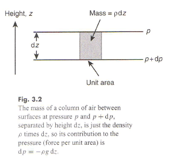
That leads to the equation of hydrostatic balance equating the pressure gradient force to the gravitational force:

dp/dz = – mng

(here p is pressure and n is the number density of molecules – N/V for N molecules in volume V). In equilibrium n(z) is given by the Boltzmann distribution:

n(z) = c.e^(-mgz/kT);

for the ideal gas pressure is given by p = nkT, so the hydrostatic balance equation becomes:

dp/dz = k T dn/dz = k T c (-mg/kT) e^{(-g m z/kT)} = – mg c e^(-mgz/kT) = – m n(z) g

I.e. the Boltzmann distribution for this ideal gas system automatically ensures the system is in hydrostatic equilibrium.

Another approach to this sort of analysis is to look at the detailed flow of molecules near an imaginary boundary. This is done in textbook calculations of the thermal conductivity of an ideal gas, for example, where a gradient in temperature results in net flow of energy (necessarily from hotter to colder). In our system with gravitational force and pressure gradients both must be taken into account in such a calculation. Such calculations are somewhat complex and depend on assumptions about molecular size and neglecting other interactions that would make the gas non-ideal, but the net effect must always satisfy the same thermodynamic laws as every other such system: in thermodynamic equilibrium temperature is uniform and there is no net energy flow through any imagined boundary.

In conclusion, after sufficient time that statistical properties cease changing, all these examples of a system with a Venus-like atmosphere must reach essentially the same isothermal or near-isothermal state. The gravitational field and adiabatic lapse rate cannot explain the high surface temperature on Venus if incoming solar radiation does not reach (at least very close to) the surface.

_____________________________________________________________________

By Leonard Weinstein

Solar Heating and Outgoing Radiation Balances for Earth and Venus

The basic heating mechanism for any planetary atmosphere depends on the balance and distribution of absorbed solar energy and outgoing radiated thermal energy. For a planet like Earth, the presence of a large amount of surface water and a relatively optically transparent atmosphere to sunlight dominates where and how the input solar energy and outgoing thermal energy create the surface and atmospheric temperatures. The unequal energy flux for day and night, and for different latitudes, combined with the planet rotation result in wind and ocean currents that move the energy around.

Earth is a much more complex system than Venus for these reasons, and also due to the biological processes and to changing albedo due to changes in clouds and surface ice. The average energy balance for the Earth was previously shown by Science of Doom, but is shown in Figure 1 below for quick reference:

From Kiehl & Trenberth (1997)

The majority of solar energy absorbed by the Earth directly heats the land and water. Some water evaporation carries this energy to higher altitudes, and is released by phase change (condensation). This energy is carried up by atmospheric convection.

In addition, convective heat transfer from the ground and oceans transfers energy to the atmosphere. It is the basic atmospheric temperature differences from day and night and at different latitude that creates pressure differences that drive the wind patterns that eventually mix and transport the atmosphere, but the buoyancy of heated air from the higher temperature surface areas also aids in the vertical mixing.

This energy is carried by convection up into the higher levels of the atmosphere and eventually radiates to space. The combination of convection of water vapor and surface heated air upwards dominates the total transported energy from the ground level. In addition, some of the ground level thermal energy is radiated up, with a portion of the thermal radiation passing directly from the ground to space. Water vapor, CO2, clouds, aerosols, and other greenhouse gases also absorb some of this radiated energy, and slightly increase the lower atmosphere and ground temperatures with back radiation effectively adding to the initial radiation, resulting in a reduced net radiation flux. This results in a higher temperature atmosphere and ground than without these absorbing materials.

Venus, however, is dominated by direct absorption of solar energy into the atmosphere (including clouds) rather than by the surface, so has a significantly different path to heat the atmosphere and ground. Venus has a very dense atmosphere (about 93 times the mass as Earth’s atmosphere), which extends to about 90 km altitude before the tropopause is reached. This is much higher than the Earth’s atmosphere.

Very dense clouds, composed mostly of sulfuric acid, reach to about 75 km, and cover the planet. The clouds have virga beneath them due to the very high temperatures at lower elevations. The clouds and thick haze occupy over half of the main troposphere height, with a fairly clear layer starting below about 30 km altitude. Due to the very high density of the atmosphere, dust and other aerosol particles (from the surface winds and possibly from volcanoes) also persist in significant quantity.

The atmosphere is 96.5% CO2, and contains significant quantities of SO2 (150 ppm), and even some H2O (20 ppm), and CO (17 ppm). These, along with the sulfuric acid clouds, dust, and other aerosols, absorb most of the incoming sunlight that is not reflected away, and also absorb essentially all of the outgoing long wave radiation and relay it to the upper atmosphere and clouds to eventually dump it into space.

A sketch is shown in Figure 2, similar to the one used for Earth, which shows the approximate energy transfer in and out of the Venus atmosphere system. It is likely that almost all of the radiation out leaves from the top of the clouds and a short distance above, which therefore locks in the level of the atmospheric temperature at that location.

The surface radiation balance shown is my guess of a reasonable level. The top portion of the clouds reflects about 75% of incident sunlight, so that Venus absorbs an average of about 163 W/m², which is significantly less than the amount absorbed by Earth. About 50% of the available sunlight is absorbed in the upper cloud layer, and about 40% of the available sunlight is captured on the way down in the lower clouds, gases, and aerosols.

Thus an average of solar energy that reaches the surface is only about 17 W/m², and the amount absorbed is somewhat less, since some is reflected. The question naturally arises as to what is the source of wind, weather, and temperature distribution on Venus, and why is Venus so hot at lower altitudes.

Venus takes 243 days to rotate. However, continual high winds in the upper atmosphere takes only about 4 days to go completely around at the equator, so the day/night temperature variation is even less than it would have otherwise been. Other circulation cells for different latitudes (Hadley cells) and some unique polar collar circulation patterns complete the main convective wind patterns.

The solar energy absorbed by the surface is a far smaller factor than for Earth, and I am convinced it is not necessary for the basic atmospheric and ground temperature conditions on Venus. Since the effect on the atmospheres of planets from absorbed solar radiation is to locally change the atmospheric pressure that drive the winds (and ocean currents if applicable), these flow currents transport energy from one location and altitude to another. There is no specific reason the absorption and release of energy has to be from the ground to the atmosphere unless the vertical mixing from buoyancy is critical. I contend that direct absorption of solar energy into the atmosphere can accomplish the mixing, and this along with the fact that the top of the clouds and a short distance above is where the radiation leaves from, is in fact the cause of heating for Venus.

We observed that unlike Earth, which had about 72% of the absorbed solar energy heat the surface, Venus has 10% or less absorbed by the ground. Also the surface temperature of Venus (about 735 K) would result in a radiation level from the ground of about 16,600 W/m².

Since back radiation can’t exceed radiation up if the ground is as warm or warmer than the atmosphere above it, the only thing that can make the ground any warmer than the atmosphere above it is the ~17 W/m² (average) from solar radiation. The ground absorbed solar radiation plus absorbed back radiation has to equal the radiation out for constant temperature. If the absorbed solar radiation were all used to heat the ground, and the net radiation heat transfer was near zero (the most extreme case of greenhouse gas blocking possible), the average temperature of the ground would only be about 0.19 K warmer than the atmosphere above it, and the excess heat would need to be removed by surface convective driven heat transfer. The buoyancy would be extremely small, and contribute little to atmospheric mixing.

However, the net radiation heat transfer out of the ground is almost surely equal to or larger than the average solar heating at the ground, from some limited transmission windows in the gas, and through a small net radiation flux. The most likely effect is that the ground is equal to or a small amount cooler than the lower atmosphere, and there is probably no buoyancy driven mixing. This condition would actually require some convective driven heat transfer from the atmosphere to the ground to maintain the ground temperature. Since the measured lower atmosphere and ground temperature are on the dry adiabatic lapse rate curve projected down from the temperature at the top of the cloud layer, the net ground radiation flux is probably close to the value of 17 W/m². This indicates that direct solar heating of the ground is almost certainly not a source for producing the winds and temperature found on Venus. The question still remains: what does cause the winds and high temperatures found on Venus?

The main point I am trying to make in this discussion is that the introduction of solar energy into the relatively cool upper atmosphere of Venus, along with the high altitude location of outgoing radiation, are sufficient to heat the lower atmosphere and surface to a much higher temperature even if no solar energy directly reaches the surface. Two simplified models are discussed in the following sections to support the plausibility of that claim. This issue is important because it relates to the mechanism causing greenhouse gas atmospheric warming, and the effect of changing amounts of the greenhouse gases.

The Tall Room

The first model is an enclosed room on Venus that is 1 km x 1km x 100 km tall. This was selected to point out how adiabatic compression can cause a high temperature at the bottom of the room, with a far lower input temperature at the top. This is the type of effect that dominates the heating on Venus. While the first part of the discussion is centered on that room model, the analysis is also applicable for part the second model, which examines a special simplified approximation of the full dynamics on Venus.

The conditions for the tall room model are:
1) A gas is introduced at the top of a perfectly thermally insulated fully enclosed room 1 km x 1 km x 100 km tall, located on the surface of Venus. The walls (and bottom and top) are assumed to have negligible heat capacity. The walls and bottom and top are also assumed to be perfect mirrors, so they do not absorb or emit radiation.

2) The supply gas temperature is selected to be 250 K. The gas pours in to fill all of the volume of the room. Sufficient quantity of gas is introduced so that the final pressure at the top of the room is at 0.1 bar at the end of inflow. The entry hole is sealed immediately after introduction of the gas is complete.

3) The gas is a single atom molecule gas such as Argon, so that it does not absorb or emit thermal radiation. This made the problem radiation independent. I also put in a qualifier, to more nearly approximate the actual atmosphere, that the gas had a C_p like that of CO2 at the surface temperature of Venus [i.e., C_p=1.14 (kJ/kg K) for CO2 at 735 K]. C_p is also temperature independent.

The room height selected would actually result in a hotter ground level than the actual case of Venus. This was due to the choice of a room 100 km tall. The height to 0.1 bar for Venus is only about 65 km, which would give a better temperature match, but the difference is not important to the discussion. A dry adiabatic lapse rate forms as the gas is introduced due to the adiabatic compression of the gas at the lower level. The value of the lapse rate for the present example comes from a NASA derivation at the Planetary Atmospheres Data Node:
http://atmos.nmsu.edu/education_and_outreach/encyclopedia/adiabatic_lapse_rate.htm
The final result for the dry adiabatic lapse rate is:

Γ_p = -dT/dz|a = g/C_p (1)

In the room at Venus, this results in:

T_H =T_top +H * 8.9/1.14 (2)

Where H is distance down from the top.

T_top remains at 250 K since it is not compressed (not because it was forced to be at that temperature by heat transfer), and T_bottom=1,031 K due to the adiabatic compression.

Two questions arise:
1) Is this dry adiabatic lapse rate what would actually develop initially after all the gas is introduced?
2) What would happen when the system comes to final equilibrium (however long it takes)?

The gas coming in would initially spread down to the bottom due to a combination of thermal motion and gravity, but the converted potential energy due to gravity over the room height would add considerable downward velocity, and this added downward velocity would convert to thermal velocity by collisions. Once enough gas filled the room to limit the MFP, added gas would tend to stay near the top until additional gas piled on top pushed it downwards, and this would increasingly compress the gas below from its added mass. The adiabatic compression of gas below the incoming gas at the top would heat the gas at the bottom to 1,031 K for the selected model. The top temperature would remain at 250 K, and the temperature profile would vary as shown by equation (2). Thus the answer to 1) is yes.

Strong convection currents may or may not be introduced in the room, depending on how fast the gas is introduced. To simplify the model, I assume the gas flows in slowly enough so that the currents are not important. It is quite clear that the temperature profile at the end of inflow would be the adiabatic lapse rate, with the top at 250 K and bottom at 1,031 K. If the final lapse rate went toward zero from thermal conduction, as Arthur postulated, even he admits it would take a very long time. The question now arises- what would cause heat conduction to occur in the presence of an adiabatic lapse rate? i.e., why would an initial adiabatic lapse rate tend to go toward an isothermal lapse rate if there is no radiation forcing (note: this lack of radiation forcing assumption is for the room model only). The cause proposed by Arthur and Science of Doom is based on their understanding of the Zeroth Law of Thermodynamics. They say that if there is a finite lapse rate (i.e., temperature gradient), there has to be conduction heat transfer. This arises from not considering the difference between temperature and heat. This is discussed in:
http://zonalandeducation.com/mstm/physics/mechanics/energy/heatAndTemperature/heatAndTemperature.html (difference between temperature and heat)

When we consider if there will be heat conduction in the atmosphere, we need to look at potential temperature rather than temperature. This is discussed at: http://en.wikipedia.org/wiki/Potential_temperature
The potential temperature is shown to be:

(3)

This term in (3) is general, and thus valid for Venus, if the appropriate pressures are used.

A good discussion why the potential temperature is appropriate to use rather than the local temperature can be found at:
https://courseware.e-education.psu.edu/simsphere/workbook/ch05.html

This includes the following statements:

• “if we return to the classic conduction laws and our discussion of resistances, we note that heat should be conducted down a temperature gradient. Since we are talking about sensible heat, the appropriate gradient for the conduction of sensible heat is not the temperature but the potential temperature. The potential temperature is simply a temperature normalized for adiabatic compression or expansion”
• “When the environmental lapse rate is exactly dry adiabatic, there is zero variation of potential temperature with height and we say that the atmosphere is in neutral equilibrium. Under these conditions, a parcel of air forced upwards (downwards) will stay where it is once moved, and not tend to sink or rise after released because it will have cooled (warmed) at exactly the same rate as the environment”.

The above material supports the claim that there would be no movement from a dry adiabatic lapse rate toward an isothermal gas in the room model.

If the initial condition was imposed– that the lapse rate was below the dry adiabatic lapse rate, it is true that the gas would be very stable from convective mixing due to buoyancy, and the very slow thermal conduction, which would drive the temperature back toward the dry adiabatic lapse rate, could take a very long time (in the actual case, it would be much faster due to even small natural convection currents generally present). However, there is no reason for any lapse rate other than the dry adiabatic lapse rate to initially form, as the problem was posed, so that issue is not even relevant.

The final result of the room model is the fact that a very high ground temperature was produced from a relative cool supply gas due to adiabatic compression of the supply that was introduced at a high altitude. This is actually a consequence of gravitational potential energy being converted to kinetic energy. Once the dry adiabatic lapse rate formed, any small flow up or down stays in temperature equilibrium at all heights, so this is a totally stable situation, and would not tend toward an isothermal situation.

If there were present a sufficient quantity of gas in the present defined room that radiated and absorbed in the temperature range of the model, the temperature would tend toward isothermal, but that was not how the tall room example was defined.

Effect of an Optical Barrier to Sunlight reaching the Ground

The second model I discussed with Science of Doom, Arthur, and others, relates to my suggestion that if an optical barrier prevented any solar energy from transmitting to the ground, but that the energy was absorbed in and heated a thin layer just below the average location of effective outgoing radiation from Venus, in such a way that the heat was transmitted downward through the atmosphere, this could also result in the hot lower atmosphere and surface that is actually observed. The albedo, and the solar heating input due to day and night, and to different latitudes, was selected to match the actual values for Venus, and the radiation out was also selected to match the values for the actual planet.

This problem is much more complicated than the enclosed room case for two reasons.

The first is that it is a dynamic and non-uniform case. The second is due to the fact that the actual atmosphere is used, with radiation absorption and emission, and the presence of clouds. The lower atmosphere and surface of the planet Venus are much hotter than for the Earth, even though the planet does not absorb as much solar energy as the Earth. It is closer to the Sun than Earth, but has a much higher albedo due to a high dense cloud layer composed mostly of sulfuric acid drops. The discussion will not attempt to examine the historical circumstances that led up to the present conditions on Venus, but only look at the effect of the actual present conditions.

In order to examine this model, I had postulated that if all of the solar heating was absorbed near the top of Venus’s atmosphere, but with the day and night and latitude variation, the heat transfer to the atmosphere downward would eventually be mixed through the atmosphere and maintain the adiabatic lapse rate, with the upper atmosphere held to the same temperature as at the present. Since the atmosphere has gases, clouds, and aerosols that absorb and radiate most if not all of the thermal radiation, this is a different problem from the tall room.

However, it appears that the radiation flux levels are relatively small, especially at lower levels, so the issue hinges on the relative amount of forcing by convective flow compared to net radiation up (which does tend to reduce the lapse rate). I use the actual temperature profile as a starting point to see if the model is able to maintain the values. Different starting profiles would complicate the discussion, but if the selected initial profile can be maintained, it is likely all reasonable initial profiles would tend to the same long-term final levels.

The assumption that the solar heating and radiation out all occur in a layer at the top of the atmosphere eliminates positive buoyancy as a mechanism to initially couple the solar energy to the atmosphere. However, the direct thermal heat-transfer with different amounts of heating and cooling at different locations causes some local expansion and contraction of different locations of the top of the atmosphere, and this causes some pressure driven convection to form.

The pressure differences from expansion and contraction set a flow in motion that greatly increases surface heat transfer, and this flow would become turbulent at reasonable induced flow speeds. This increases heat transfer and mixing to larger depths. The portions cooler than the local average atmosphere will be denser than local adiabatic lapse rate values from the average atmosphere, and thus negative buoyancy would cause downward flow at these locations.

As the flow moved downward, it compressed but initially remains slightly cooler than the surrounding, with some mixing and diffusion spreading the cooling to ever-larger volumes. At some level, the flow down actually passes into a surrounding volume that is slightly cooler, rather than warmer, than the flow, due to the small but finite radiation flux removing energy from the surrounding. At this point the downward flow stream is warming the surrounding. The question arises: how much energy is carried by the convection, and could it easily replace radiated energy, so as to maintain a level near the dry adiabatic lapse rate?

A few numbers need to be shown here to best get an order of magnitude of what is going on. Arthur has already made some of these calculations. The average input energy of 158 W/m² applied to Venus’s atmosphere would take about 100 years to change the average atmospheric temperature by 500 K. This means that to change it even 0.1 K (on average) would take about 7 days. Since the upper atmosphere at low latitudes only takes about 4 days to completely circulate around Venus, the temperature variations from average values would be fairly small if the entire atmosphere were mixed.

However, for the model proposed, only a very thin layer would be heated and cooled under the absorbing layer. Differences in net radiation flux would also help transfer energy up and down some. This relatively thin layer would thus have much higher temperature variation than the average atmosphere mass would (but still only a few degrees). The pressure variations due to the upper level temperature variations would cause some flow circulation and vertical mixing to occur throughout the atmosphere. The circulating flows may or may not carry enough energy to overcome radiation flux levels to maintain the dry adiabatic lapse rate. Let us look at the near surface flow, and a level of radiation flux of 17 W/m².

What excess temperature and vertical convection speed is needed to carry energy able to balance that flux level. Assume a temperature excess of only 0.026 K is carried and mixed by convection due to atmospheric circulation. Also assume the local horizontal flow rate near the ground is 1 m/s. If a vertical mixing of only 0.01 m/s were available, the heat added would be 17 W/m², and this would balance the lost energy due to radiation, thus allowing the dry adiabatic lapse rate to be maintained.

This shows how little convective circulation and mixing are needed to carry solar heated atmosphere from high altitudes to lower levels to replace energy lost by radiation flux levels in the atmosphere, and maintain a near dry adiabatic lapse rate. It is the solar radiation that is supplying the input energy, and adiabatic compression that is heating the atmosphere. As long as the lapse rate is held close to the adiabatic level with sufficient convective mixing, it is the temperature at the location in the atmosphere where the effective outgoing radiation is located that sets a temperature on the adiabatic lapse rate curve and adiabatic compression determines the lower atmosphere temperature.

Since the exact details of the heat exchanges are critical to the process, this optically sealed region near the top of the atmosphere is a poorly defined model as it stands, and the question of whether it actually would work as Arthur and Science of Doom question is not resolved, although an argument can be made that there are processes to do the mixing. However, the real atmosphere of Venus absorbs almost all of the solar energy in its upper half, and this much larger initial absorption volume does clearly do the job. I have shown the ground likely has little if any effect on the actual temperature on Venus.

Some Concluding Remarks

The initial cause for this discussion was the question of why the surface of Venus is as hot as it is. A write-up by Steve Goddard implied that the high pressure on Venus was a major factor, and even though some greenhouse gas was needed to trap thermal energy, it was the pressure that was the major contributor. The point was that an adiabatic lapse rate would be present with or without a greenhouse gas, and the major effect of the greenhouse gas was to move the location of outgoing radiation to a high altitude. The outgoing level set a temperature at that altitude, and the ground temperature was just the temperature at the outgoing radiation effective level plus the increase due to adiabatic compression to the ground. The altitude where the effective outgoing radiation occurs is a function of amount and type of greenhouse gases. Steve’s statement is almost valid. If he qualified it to state that enough greenhouse gas is still needed to limit the radiation flux, and keep the outgoing radiation altitude near the top of the atmosphere, he would have been correct. Thus both the amount of atmosphere (and thus pressure and thickness), and amount of greenhouse gases are factors. Any statement that greenhouse gases are not needed if the pressure is high enough is wrong (but this was not what Steve Goddard said).

Another issue that came up was the need for the solar energy to heat the ground in order for the hot surface of Venus to occur. I think I made reasonable arguments that this is not at all true. While there is a small amount of solar heating of the ground, the ground is probably actually slightly cooler that the atmosphere directly above it due to radiation, and so there is no buoyant mixing and no heating of the atmosphere from the ground other than the small radiated contribution. The main part of solar energy is absorbed directly into the atmosphere and clouds, and is almost certainly the driver for winds and mixing, and the high ground temperature.

The final issue is what would happen if most (say 90%) of the CO2 were replaced by say Argon in Venus’s atmosphere. Three things would happen:

1) The adiabatic lapse rate would greatly increase due to the much lower Cp of Argon.

2) The height of the outgoing radiation would probably decrease, but likely not much due to both the presence of the clouds, and the fact that the density is not linear with altitude, and matching a height with remaining high CO2 level would only drop 10 to 15 km out of the 75 to 80, where outgoing radiation is presently from. If in fact it is the clouds that cause most of the outgoing radiation, there may not be any drop in outgoing level.

3) The radiation flux through the atmosphere would increase, but probably not nearly enough to prevent the atmospheric mixing from maintaining an adiabatic lapse rate. Keep in mind that Venus has 230,000 times the CO2 as Earth. Even 10% of this is 23,000 times the Earth value.

The combination of these factors, especially 1), would probably result in an increase in the ground temperature on Venus.

Read Full Post »

References

Broadband reflectance and emissivity of specular and rough water surfaces, Sidran, Applied Optics (1981)
In situ angular measurements of thermal infrared sea surface emissivity—validation of models, Niclòs, Valor, Caselles, Coll & Sànchez, Remote Sensing of Environment (2005)
Measurement of the Sea Surface Emissivity, Konda, Imasato, Nishi and Toda, Journal of Oceanography (1994)
Observations of the Infrared Radiative Properties of the Ocean—Implications for the Measurement of Sea Surface Temperature via Satellite Remote Sensing, Smith, Knuteson, Revercomb, Feltz, Nalli, Howell, Menzel, Brown, Brown, Minnett & McKeown, Bulletin of the American Meteorological Society (1996)
The polarized emissivity of a wind-roughened sea surface: A Monte Carlo model, Henderson, Theiler & Villeneuve, Remote Sensing of Environment (2003)
Notes
Note 1: The upward radiation from the surface is the sum of three contributions: (i) direct emission of the sea surface, which is attenuated by the absorption of the atmospheric layer between the sea surface and the instrument; (ii) reflection of the downwelling sky radiance on the sea, attenuated by the atmosphere; and (iii) the upwelling atmospheric radiance emitted in the observing direction.
So the measured radiance can be expressed as:
where the three terms on the right are each of the three contributions noted in the same order.
Note 2: 1/10th of the search results returned from one journal for the search term “emissivity sea surface”:
Remote Sensing of Environment - search results
Atmospheric Radiation: Theoretical Basis, Goody & Yung, Oxford University Press (2nd ed. 1989)
How Dry is the Tropical Free Troposphere? Implications for Global Warming Theory,
Spencer & Braswell, Bulletin of the American Meteorological Society (1997)
Humidity-Temperature Relationships in the Tropical Troposphere, Sun & Oort, Journal of Climate (1995)
Distribution of Tropical Tropospheric Water Vapor, Sun & Lindzen, Journal of Atmospheric Sciences (1993)
Sensitivity of the Earth’s Climate to height-dependent changes in the water vapor mixing ratio, Shine & Sinha, Nature (1991)
Some Coolness concerning Global Warming, Lindzen,Bulletin of the American Meteorological Society (1990)
Note 1 – The total amount of water vapor, TPW ( total precipitable water), is obviously something we want to know, but we don’t have enough information if we don’t know the distribution of this water vapor with height. It’s a shame, because TPW is the easiest value to measure via satellite.
Note 2 – Obviously the total mass of air is conserved. If small areas have rapidly rising air, larger areas will have have slower subsiding air.
Frontiers of Climate Modeling, ed. J.T. Kiehl & V. Ramanathan, Cambridge University Press (2006)
Water Vapor Feedback and Global Warming, I.M. Held & B.J. Soden, Annual Review of Energy and the Environment (2000)