In Ensemble Forecasting I wrote a short section on parameterization using the example of latent heat transfer and said:
Are we sure that over Connecticut the parameter CDE = 0.004, or should it be 0.0035? In fact, parameters like this are usually calculated from the average of a number of experiments. They conceal as much as they reveal. The correct value probably depends on other parameters. In so far as it represents a real physical property it will vary depending on the time of day, seasons and other factors. It might even be, “on average”, wrong. Because “on average” over the set of experiments was an imperfect sample. And “on average” over all climate conditions is a different sample.
Interestingly, a new paper has just shown up in JGR (“accepted for publication” and on their website in the pre-publishing format): Seasonal changes in physical processes controlling evaporation over an inland water, Qianyu Zhang & Heping Liu.
They carried out detailed measurements over a large reservoir (134 km² and 4-8m deep) in Mississippi for the winter and summer months of 2008. What were they trying to do?
Understanding physical processes that control turbulent fluxes of energy, heat, water vapor, and trace gases over inland water surfaces is critical in quantifying their influences on local, regional, and global climate. Since direct measurements of turbulent fluxes of sensible heat (H) and latent heat (LE) over inland waters with eddy covariance systems are still rare, process-based understanding of water-atmosphere interactions remains very limited..
..Many numerical weather prediction and climate models use the bulk transfer relations to estimate H and LE over water surfaces. Given substantial biases in modeling results against observations, process-based analysis and model validations are essential in improving parameterizations of water-atmosphere exchange processes..
Before we get into their paper, here is a relevant quote on parameterization from a different discipline. This is from Turbulent dispersion in the ocean, Garrett (2006):
Including the effects of processes that are unresolved in models is one of the central problems in oceanography.
In particular, for temperature, salinity, or some other scalar, one seeks to parameterize the eddy flux in terms of quantities that are resolved by the models. This has been much discussed, with determinations of the correct parameterization relying on a combination of deductions from the large-scale models, observations of the eddy fluxes or associated quantities, and the development of an understanding of the processes responsible for the fluxes.
The key remark to make is that it is only through process studies that we can reach an understanding leading to formulae that are valid in changing conditions, rather than just having numerical values which may only be valid in present conditions.
[Emphasis added]
Background
Latent heat transfer is the primary mechanism globally for transferring the solar radiation that is absorbed at the surface up into the atmosphere. Sensible heat is a lot smaller by comparison with latent heat. Both are “convection” in a broad term – the movement of heat by the bulk movement of air. But one is carrying the “extra heat” of evaporated water. When the evaporated water condenses (usually higher up in the atmosphere) it releases this stored heat.
Let’s take a look at the standard parameterization in use (adopting their notation) for latent heat:
LE = ρaLCEU(qw −qa)
LE = latent heat transfer, ρa = air density, L = latent heat of vaporization (2.5×10⁶ J kg–1), CE = bulk transfer coefficient for moisture, U = wind speed, qw & qa are the respective specific humidity in the water-atmosphere interface and the over-water atmosphere
The values ρa and L are a fundamental values. The formula says that the key parameters are:
- wind speed (horizontal)
- the difference between the humidity at the water surface (this is the saturated value which varies strongly with temperature) and the humidity in the air above
We would expect the differential of humidity to be important – if the air above is saturated then latent heat transfer will be zero, because there is no way to move any more water vapor into the air above. At the other extreme, if the air above is completely dry then we have maximized the potential for moving water vapor into the atmosphere.
The product of wind speed and humidity difference indicate how much mixing is going on due to air flow. There is a lot of theory and experiment behind the ideas, going back into the 1950s or further, but in the end it is an over-simplification.
That’s what all parameterizations are – over-simplifications.
The real formula is much simpler:
LE = ρaL<w’q’>, where the brackets denote averages,w’q’ = the turbulent moisture flux
w is the upwards velocity, q is moisture; and the ‘ denoting eddies
Note to commenters, if you write < or > in the comment it gets dropped because WordPress treats it like a html tag. You need to write < or >
The key part of this equation just says “how much moisture is being carried upwards by turbulent flow”. That’s the real value so why don’t we measure that instead?
Here’s a graph of horizontal wind over a short time period from Stull (1988):

From Stull 1988
Figure 1
And any given location the wind varies across every timescale. Pick another location and the results are different. This is the problem of turbulence.
And to get accurate measurements for the paper we are looking at now, they had quite a setup:
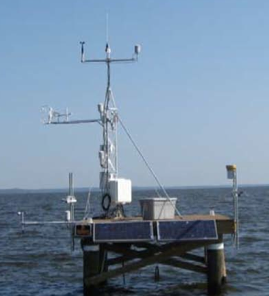
Figure 2
Here’s the description of the instrumentation:
An eddy covariance system at a height of 4 m above the water surface consisted of a three-dimensional sonic anemometer (model CSAT3, Campbell Scientific, Inc.) and an open path CO2/H2O infrared gas analyzer (IRGA; Model LI-7500, LI-COR, Inc.).
A datalogger (model CR5000, Campbell Scientific, Inc.) recorded three-dimensional wind velocity components and sonic virtual temperature from the sonic anemometer and densities of carbon dioxide and water vapor from the IRGA at a frequency of 10 Hz.
Other microclimate variables were also measured, including Rn at 1.2 m (model Q-7.1, Radiation and Energy Balance Systems, Campbell Scientific, Inc.), air temperature (Ta) and relative humidity (RH) (model HMP45C, Vaisala, Inc.) at approximately 1.9, 3.0, 4.0, and 5.5 m, wind speeds (U) and wind direction (WD) (model 03001, RM Young, Inc.) at 5.5 m.
An infrared temperature sensor (model IRR-P, Apogee, Inc.) was deployed to measure water skin temperature (Tw).
Vapor pressure (ew) in the water-air interface was equivalent to saturation vapor pressure at Tw [Buck, 1981].
The same datalogger recorded signals from all the above microclimate sensors at 30-min intervals. Six deep cycling marine batteries charged by two solar panels (model SP65, 65 Watt Solar Panel, Campbell Scientific, Inc.) powered all instruments. A monthly visit to the tower was scheduled to provide maintenance and download the 10-Hz time-series data.
I don’t know the price tag but I don’t think the equipment is cheap. So this kind of setup can be used for research, but we can’t put one each every 1km across a country or an ocean and collect continuous data.
That’s why we need parameterizations if we want to get some climatological data. Of course, these need verifying, and that’s what this paper (and many others) are about.
Results
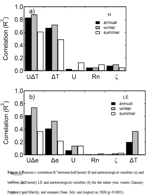
When we look back at the parameterized equation for latent heat it’s clear that latent heat should vary linearly with the product of wind speed and humidity differential. The top graph is sensible heat which we won’t focus on, the bottom graph is latent heat. Δe is humidity, expressed as partial pressure rather than g/kg. We see that the correlation between LE and wind speed x humidity differential is very different in summer and winter:
From Zhang & Liu 2014
Figure 2
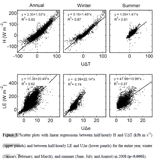
The scatterplots showing the same information:
From Zhang & Liu 2014
Figure 3
The authors looked at the diurnal cycle – averaging the result for the time of day over the period of the results, separated into winter and summer.
Our results also suggest that the influences of U on LE may not be captured simply by the product of U and Δe [humidity differential] on short timescales, especially in summer. This situation became more serious when the ASL (atmospheric surface layer, see note 1) became more unstable, as reflected by our summer cases (i.e., more unstable) versus the winter cases.
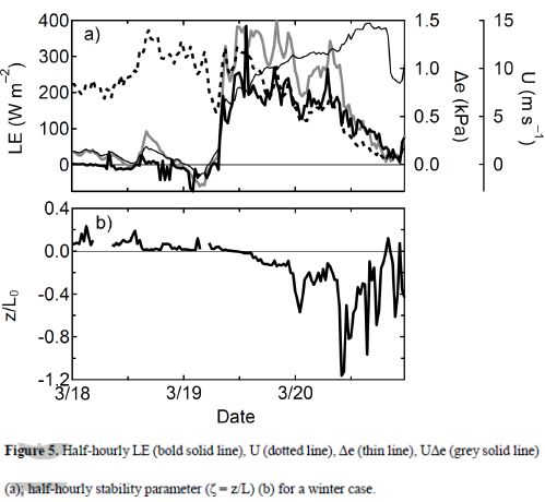
They selected one period to review in detail. First the winter results:
From Zhang & Liu 2014
Figure 4
On March 18, Δe was small (i.e., 0 ~ 0.2 kPa) and it experienced little diurnal variations, leading to limited water vapor supply (Fig. 5a).
The ASL (see note 1) during this period was slightly stable (Fig. 5b), which suppressed turbulent exchange of LE. As a result, LE approached zero and even became negative, though strong wind speeds of approximately around 10 ms–1 were present, indicating a strong mechanical turbulent mixing in the ASL.
On March 19, with an increased Δe up to approximately 1.0 kPa, LE closely followed Δe and increased from zero to more than 200 Wm–2. Meanwhile, the ASL experienced a transition from stable to unstable conditions (Fig. 5b), coinciding with an increase in LE.
On March 20, however, the continuous increase of Δe did not lead to an increase in LE. Instead, LE decreased gradually from 200 Wm–2 to about zero, which was closely associated with the steady decrease in U from 10 ms–1 to nearly zero and with the decreased instability.
These results suggest that LE was strongly limited by Δe, instead of U when Δe was low; and LE was jointly regulated by variations in Δe and U once a moderate Δe level was reached and maintained, indicating a nonlinear response of LE to U and Δe induced by ASL stability. The ASL stability largely contributed to variations in LE in winter.
Then the summer results:
From Zhang & Liu 2014
Figure 5
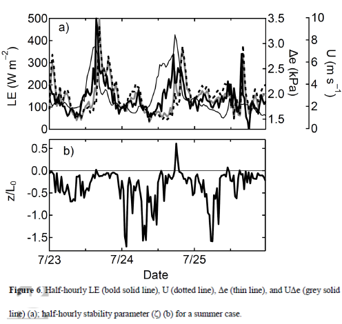
In summer (i.e., July 23 – 25 in Fig. 6), Δe was large with a magnitude of 1.5 ~ 3.0 kPa, providing adequate water vapor supply for evaporation, and had strong diurnal variations (Fig. 6a).
U exhibited diurnal variations from about 0 to 8 ms–1. LE was regulated by both Δe and U, as reflected by the fact that LE variations on the July 24 afternoon did not follow solely either the variations of U or the variations of Δe. When the diurnal variations of Δe and U were small in July 25, LE was also regulated by both U and Δe or largely by U when the change in U was apparent.
Note that during this period, the ASL was strongly unstable in the morning and weakly unstable in the afternoon and evening (Fig. 6b), negatively corresponding to diurnal variations in LE. This result indicates that the ASL stability had minor impacts on diurnal variations in LE during this period.
Another way to see the data is by plotting the results to see how valid the parameterized equation appears. Here we should have a straight line between LE/U and Δe as the caption explains:
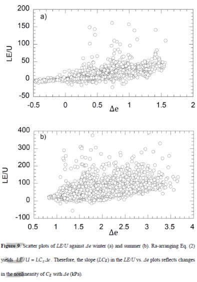
From Zhang & Liu 2014
Figure 6
One method to determine the bulk transfer coefficients is to use the mass transfer relations (Eqs. 1, 2) by quantifying the slopes of the linear regression of LE against UΔe. Our results suggest that using this approach to determine the bulk transfer coefficient may cause large bias, given the fact that one UΔe value may correspond to largely different LE values.
They conclude:
Our results suggest that these highly nonlinear responses of LE to environmental variables may not be represented in the bulk transfer relations in an appropriate manner, which requires further studies and discussion.
Conclusion
Parameterizations are inevitable. Understanding their limitations is very difficult. A series of studies might indicate that there is a “linear” relationship with some scatter, but that might just be disguising or ignoring a variable that never appears in the parameterization.
As Garrett commented “..having numerical values which may only be valid in present conditions”. That is, if the mean state of another climate variable shifts the parameterization will be invalid, or less accurate.
Alternatively, given the non-linear nature of climate process, changes don’t “average out”. So the mean state of another climate variable may not shift, the mean state might be constant, but its variation with time or another variable may introduce a change in the real process that results in an overall shift in climate.
There are other problems with calculating latent heat transfer – even accepting the parameterization as the best version of “the truth” – there are large observational gaps in the parameters we need to measure (wind speed and humidity above the ocean) even at the resolution of current climate models. This is one reason why there is a need for reanalysis products.
I found it interesting to see how complicated latent heat variations were over a water surface.
References
Seasonal changes in physical processes controlling evaporation over an inland water, Qianyu Zhang & Heping Liu, JGR (2014)
Turbulent dispersion in the ocean, Chris Garrett, Progress in Oceanography (2006)
Notes
Note 1: The ASL (atmospheric surface layer) stability is described by the Obukhov stability parameter:
ζ = z/L0
where z is the height above ground level and L0 is the Obukhov parameter.
L0 = −θvu*3/[kg(w’θv‘)s ]
where θv is virtual potential temperature (K), u* is frictional velocity by the eddy covariance system (ms–1), k is Von Karman constant (0.4), g is acceleration due to gravity (9.8 ms–2), w is vertical velocity (m s–1), and (w’θv‘)s is the flux of virtual potential temperature by the eddy covariance system


This looks like far better instrumentation for determining sensible and latent heat transfer than was used in the EBEX experiment. Too bad they didn’t put a set of radiometers on the platform too.
They did measure net radiation. Here’s the diurnal value of everything, averaged over the time period of the measurements, and separated into the two seasons:
Did they do an energy balance for the year? I can see a problem, though, that wouldn’t happen on land: horizontal energy flow from water currents.
DeWitt,
No they didn’t comment on an energy balance.
I noticed that at lest Rn is left undefined in the post. The article defines the variable in the introduction:
I would describe the situation rather by noting that H and LE react very strongly to local conditions and thus force ΔT and Δe to their relatively small values over small distances in spite of the large diurnal variation of solar heating. In other words these variables are strongly linked, but telling which is the driver and which driven is less obvious.
Another factor that reduces the influence of the diurnal Rn variability on other variables is the penetration of SW to layers below the skin. Only a fraction of SW is absorbed very close to the skin.
There’s a huge literature on the Penman and Penman-Monteith equations for the flux density of latent heat. I’ve collected a few here: https://www.dropbox.com/sh/hgxtblg209q075t/AAAoaeXUpowFPhlWC7gi08XXa Or a Google / Google Scholar search will lead you to many. Or a search at the AMS Journals site http://journals.ametsoc.org/ .
For a closer look at the physical phenomena and processes occurring at the interface, a search with S. Banerjee as author and key words like turbulence. air-water interface, gas-liquid interface, scalar exchange, & etc. will also work. Professor Banerjee has a partial list of publications online here: cuny.edu/site/energy/faculty-research/sbanerjee/recent-publications.html a few of which address geophysical applications.
Dan,
I had a look at a few papers and also at one of the source papers, Evaporation and environment, JL Monteith, Symp. Soc. Exp. Biol, (1965).
It seems this application is a little different, primarily water evaporating out of plants.
I think that’s why the formula is different.
With plants, wind speeds have an effect but there’s a limiting factor in the plant – whereas open water surfaces offer an unlimited supply of water and the limitation is the “sink” of unsaturated air above.
At least, that’s my take on the difference. I would be interested if you had any comments.
SoD, I’m on the clock for a while and will get back to this a little later.
SOD: I’m a little confused about what process this equation is meant to describe in a GCM:
LE = ρ_a*L*CE*U*(q_w −q_a)
If it described evaporation from liquid water to water vapor, I would expect to see a term for temperature. (q_w does vary with temperature.) The rate of evaporation depends on the rate at which water molecules escape the liquid phase, which presumably depends on temperature, surface area and the pressure of air above. And the NET rate of evaporation depends on the rate at which water vapor is returning to the liquid phase.
It seems likely that this equation is describing transport of the latent heat in water vapor into the atmosphere from a thin layer of air above the surface of the water. The water vapor in this thin layer is assumed to be in equilibrium (saturated) with the liquid water below, so the effect of water temperature has already been included in q_w. In this case, this equation would describe latent heat transport from one location in the atmosphere (a thin layer above the ocean) to another location, but the identity of the second location is also unclear. Perhaps it is simply the lowest grid cell of the atmosphere.
If I am correct so far, this equation covers the latent heat lost by the surface layer of the water, even though the equation itself describes transport of water vapor within the atmosphere.
Changing the subject: Why do we expect that vertical transport of water vapor to vary linearly with horizontal wind speed? Is this standard turbulent mixing?
Frank,
The physical idea behind this formula is that water molecules exit and enter the surface always at a high enough rate to maintain saturation humidity in the immediate neighborhood of the surface. As long as this is true the rates of those balancing processes do not matter. Therefore the temperature enters the equation only true it’s influence on the variables shown. The influence on qw (and on ρa) is direct, while qa and U are influenced indirectly.
The other location is defined to be at the reference height. The main reference height was 5.5 m in the measurements reported by Zhang and Liu, but they made part of the measurements also at lower heights.
Pekka: Thanks for the reply. I looks like I understood most of this. If I understand correctly from Issac Held’s post on this subject, the relative humidity at the reference height averages 80% and the specific humidity remains constant above that in the boundary layer (unless the condensation level is reached). So it looks like a lot is changing in the first few meters or less above the surface (100% to 80% relative humidity) and not much changes above.
If I rearrange the terms a little:
LE = ρ_a*L*CE*U*q_w*(1 − q_a/q_w)
LE = ρ_a*L*CE*U*q_w*(1 − RH)
LE = ρ_a*L*CE*U*q_w*0.2
We know that q_w increases about 6-7%/degC at relevant temperatures. If 2XCO2 were to raise SST by 3 degC, convection of latent heat would increase by 20% or 16 W/m2 over the ocean. For a surface warming of 3 degC (288 to 291 degK), radiative cooling increases about 16 W/m2. However, assuming a constant lapse rate, DLR will increase nearly as much, 14 W/m2 (333 W/m2 to 347 W/m2 for a 3 degK increase assuming the atmosphere had emissivity of 1). Assuming my calculations are correct, this is an interesting demonstration of the importance of convective cooling compared with net radiative cooling.
As discussed in different terms by Issac, maintaining a surface energy balance will require U or RH to change. It would be interesting to know observations during the seasonal temperature cycle (about 3 degK) are consistent with these expectations.
Frank,
What I write in my comment above is closely related to what Isaac Held writes at the end of his post.
When we consider evaporation over oceans (or other wide areas of water rather than a relatively small reservoir) it’s ultimately the energy balance that controls what goes on. The sum of net IR, latent heat transfer and sensible heat transfer must add up to the heating by solar SW when averages over areas and periods long enough are considered, and when the small net energy flux that warm or cool the ocean in the region considered is can be neglected. The constraint set by the energy balance shifts much of the control of what’s going on to higher altitudes. In a detailed enough atmospheric model the model equations are probably good enough for handling that, but in a GCM type climate model where the grid cells are large, the role of parametrizations is likely to be essential over most relevant scales.
Pekka: If you look from the surface energy balance perspective, instantaneous doubling of CO2 produces a radiative imbalance of only about 0.8 W/m2 (DeWItt’s number). That could be balanced by a 1% increase in convected latent heat or an SST rise of 0.15 degC. The problem is that the upper troposphere will warm far more than the surface, reducing the lapse rate. So convection must go down, at least transiently, not up. So I understand your comment that the upper atmosphere is in control.
If wind speed in the tropics depends mostly on the overall speed of the Hadley circulation, the rate at which the upper troposphere cools and descends will control surface wind and thereby evaporation/latent heat. If wind speed in the tropics isn’t driven mostly by the Hadley circulation, there will be nowhere for the extra water vapor to go if wind increased. The relative humidity in the boundary layer would then rise, diminishing evaporation.
I wasn’t fully specific in my earlier comment. Therefore I explain my point a bit more.
Averaging over an large enough area lateral mass and energy transfer is much smaller than vertical and can be neglected. Then we can consider four main variables:
– temperature
– humidity
– vertical flux of sensible heat
– vertical flux of latent heat or equivalently of water vapor
Most other variables can be determined from these, but wind speed is an additional independent variable that enters the standard equations as a controlling factor.
When we consider a very low height small changes in the temperature and humidity lead to very large changes in the dynamics of the layer below this height, but to little change in the dynamics above that height.
– Looking at the layer below the height vertical fluxes at the reference height adjust easily to the new temperature and humidity, but looking at what happens above the fluxes don’t change much at all.
– Conversely forcing moderate changes in the vertical fluxes at the top of the layer below leads to relatively small changes in the temperature and humidity at the top of that layer, but forcing the same changes at the bottom of the atmosphere above leads to much larger changes in temperature and humidity.
From the above points we can conclude that the dynamics of the ocean-atmosphere system tells that the temperature and humidity at a low height are determined mainly by the properties of the surface, while the fluxes are determined by the properties of the atmosphere above that height. The equations that are essential for solving the actual values are those that describe the storage of heat in the top ocean and those that describe the dynamics of the atmosphere above the lowest heights. What happens between the surface and a low reference height simply adjusts to these more important factors without any major influence on the outcome.
Frank,
Not only might convection go down, leading to surface warming, but DLR would also increase as the lapse rate decreases. The 0.8W/m¯ increase in DLR is calculated after a change in CO2, but with no change in anything else.
That seems to be limiting yourself to a perspective taken from the surface. If the upper troposphere temperature increases, wont that increase convection in the upper troposphere driving the energy higher where it can be radiated more easily?
And if upper troposphere convection increases then so should the lower troposphere convection with a similar idea where a thunderstorm’s winds are driven from the convection created as the cloud forms.
TTTM,
Physical convection, i.e. the vertical movement of air mass, does not have to increase to increase energy transfer as the temperature goes up. The enthalpy of moist air increases rapidly as the specific humidity increases and at constant relative humidity, the specific humidity increases exponentially with temperature. So the same amount of air carries more energy. The enthalpy of moist air must include the heat of evaporation of the water as well as the heat capacity of the air.
Also, a decrease in lapse rate does not necessarily mean a decrease in convection because as the humidity increases, the moist adiabatic lapse rate also decreases. A warmer troposphere also means the tropopause moves to higher altitude because air expands as it warms.
I think in this case its mostly dry air (as opposed to “moist” air) as we’re talking about the upper troposphere. Hence I would have thought the energy should stay relatively constant.
Spencer once did a “back of the envelope” calculation on the change in the ERL due to a doubling of CO2 and it only worked out to be 60m or so.
Good question. The answer is involved. I think it’s probably better to try and explain in the next article.
And the attempted explanation in Turbulence, Closure and Parameterization
I’m back on this discussion and will address the general aspects of the Penman correlations soon.
However, when I first read the post I was struck by this sentence, “Sensible heat is a lot smaller by comparison with latent heat.” I recalled the following paper
Adrian Bejan and A. Heitor Reis, Thermodynamic optimization of global circulation and climate, Int. J. Energy Res., Vol. 29, pp. 303–316, 2005.
and this discussion in Section 4:
” 4. THE EFFECT OF EVAPORATION/CONDENSATION OF WATER IN THE ATMOSPHERE
Better agreement between the present theory and observed properties of atmospheric circulation is obtained if we account for the effect of latent heat in heating and cooling of humid air. In the analysis of Section 2, we used only the sensible heat effect. The ratio between the sensible heat and latent heat effects in the atmosphere is known as the Bowen ratio (Bo). According to Brutsaert (1991), several Bo estimates are available and are of the same order of magnitude, for example: Budyko (Bo=5), Reichel (Bo=3.8), and Korzum et al . (Bo=5.6) (cf. (Brutsaert, 1991) p. 5). The Bo effect can be added to the preceding model by dividing the right side of Equation (14) by Bo. ”
where:
Brutsaert W. 1991. Evaporation into the Atmosphere. Kluwer Academic Publishers: Dordrecht, The Netherlands.
In other words, B = H/LE, H = B * LE and therefore H > LE
The statement by Bejan and co-workers has appeared in several related papers over a period of a few years. I would be surprised if it is not correct.
According to Trenberth, Fasullo, and Kiehl the surface fluxes are 17 W/m^2 sensible and 80 W/m^2 evaporation for global averages. Stephens et al (2012) give values 24±7 W/m^2 and 88±10 W/m^2. I guess these values are the basis for SoD’s statement.
These values apply only to the surface. With increasing height latent heat transfer decreases and gets converted to sensible heat flux. Changes in the relative importance of radiative heat transfer influence also the balance as the net IR increases with altitude reaching essentially 100% at tropopause.
At the height of a few meters the net fluxes cannot differ much from the surface.
Thanks Pekka. I’ll look into the question in more detail.
Trenberth’s figure for sensible heat is CALCULATED to produce a small surface energy imbalance consistent with ocean warming. He asserts that his value is consistent with the estimates from reanalyses made by Budyko and others.
Dan,
I had a look at Bejan’s paper and there’s little definition, it’s like a throwaway line at the end of the paper, like a reviewer had said “what about if?”.
The reference: Evaporation into the Atmosphere. Kluwer Academic Publishers: Dordrecht, The Netherlands, W Brutsaert (1991) is not available to me. I did find part of a paper by the same author which interestingly commented on why the Penman model is used rather than the bulk aerodynamic formula. I can’t access the whole paper:
The Formulation of Evaporation from Land Surfaces (1991).
Anyway, it would be a bit of an over-turning of many decades of work if this ratio was as Bejan describes it for the surface.
Here is Global Physical Climatology, Dennis Hartmann (1994). By the way, I recommended this book a long time ago in Find Stuff Out and Book Reviews and I’d forgotten how good it was:
Now the Bowen ratio, Bo, is the ratio of sensible heat flux to latent heat flux from the surface. In a saturated atmosphere over a wet surface this value is called the equilibrium Bowen ratio, Be, and can be calculated:
Be = SH/LH = cp / [L(∂q*/∂T)]
where q* is the saturated humidity
At 0’C the equilibrium Bowen ratio is about 1, and at 30’C it is about 0.2
Once we remove the saturated condition and have RH < 1 then of course LH increases, so the Bowen ratio in practice, Bo < Be (equilibrium Bowen ratio).
So for water surfaces – the ocean – the Bowen ratio globally must be something between 0.2 and 1.
For dry land surfaces of course the Bowen ratio can be quite high – like over deserts.
So if we are talking about the surface flux over the globe, Bejan is surely wrong.
And if we consider it from another point of view, the latent heat flux globally can be calculated from the rainfall (what goes up must come down), which is where Kiehl & Trenberth (and others) get their data from. There’s quite a lot of uncertainty about global rainfall but not that much.
So if we take the non-radiative flux up from the surface, globally annually averaged, of about 110 W/m2 then for a Bowen ratio of 5 we would have a latent heat flux of 18 W/m2 and sensible heat flux of 92 W/m2.
Now, as I’ve written all of this, I notice that Bejan cites Budyko. Well, this is a standard old climatology reference. In fact, Hartmann cites Budyko quite often as do many other people.
Here is Hartmann citing Budyko:
Sometimes the equilibrium Bowen ratio is shown inverted: 1/Be=L/cp . (∂q*/∂T)
Perhaps Bejan has his Bowen ratio upside down. Because the standard value is about 0.2 and Bejan is quoting numbers like 5..
The Penman model is based on an energy balance at the interface between the source for the liquid water and the sink ( destination ) of the water vapor. The balance includes both radiative and convective contributions to the energy balance, and associated resistances from the source to the sink. The surface energy balance is solved for the latent-energy contribution and includes accounting for both radiative-and convective contributions to the evaporation. The papers that I linked to in my original comment cover detailed derivations, discussions, and applications of the Penman model and its variations.
The model is applied to both liquid water surfaces and surfaces comprised of vegetation. In the latter case, resistances include one associated with the radiative source of energy in addition to that for the path of the vapor from the source to the sink. In the case of some vegetation the pathway can be completely closed by mechanisms internal to the vegetation. In this case, the associated resistance will be infinite and no transvaporation ( evapotranspiration ) from the interior of the plant can occur; blind application of a bulk-to-bulk model will clearly lead to incorrect results.
The model discussed in the subject post is related to the convective component of latent-energy transport. The modeling applies the almost universal approach of a transfer coefficient times a bulk-to-bulk driving potential. In this case the transfer coefficient is related to the turbulent motions in the atmosphere near the interface. And this in turn is related to turbulence in the bulk far from the interface; generally because that’s about all we know when the critical issue is related to turbulence near a constantly-changing, compliant interface that frequently involves mists of liquid droplets from breaking waves. The actual area over which the mass flux is active is not known.
Relating the transfer coefficient to the turbulence in the atmosphere implicitly assumes that the dominate, critical, controlling resistance is solely in the atmosphere; the resistance is independent of the processes on the liquid side. The Google search for papers by Sanjoy Banerjee and co-workers that I mentioned in my original comment, instead, indicates that the controlling resistance for the case of gas transfer into a liquid is on the liquid side. A fact that has been known since the first investigations by Dankwerts in the late 1940s and early 1950s. That approach has also been successfully applied to the case of condensation of a vapor onto its liquid phase ( Google surface renewal condensation stratified ). I do not know if the approach has been teased against the evaporation case. Since about 1969, Banerjee has continued investigations and attempted to refine calculation of the transfer coefficient to the most fundamental level.
Dan,
In looking for Bejan’s source I found this extract in another paper by Bejan’s source, The Formulation of Evaporation from Land Surfaces, W Brutsaert (1991):
oops bested again by auto-suggestion, auto-completion, auto-correction.
teased == tested
Science and others,
Thanks for all the additional info. Apparently, Bejan et al. do have it upside down.
When I have been reading comments on energy budget ind higher latitudes, I have understod that it is the albedo effect that is the greatest driver. The athmosphere is seen as dry. But I am not sure that it is the truth. What will the parameter tell us about evaporation of open ocean. at air temperature of -30 C,and some breeze, let`s say 10 m/s. In cold days, over rivers, there is the phenomenon of frost smoke, that vater vapor is icing. This shows that it is evaporation even when the air is very cold..Perhaps this means that latent heat is more important than albedo in climate regulation,even near the poles, and that there is no dry atmosphere.
nobodyknows,
The operative word above is rivers. You aren’t going to have an air temperature of -30 over a large expanse of open water. In the Arctic, the near surface air temperature doesn’t reach -30 until the surface is covered with ice. But even ice with a surface temperature of -30 has a saturation vapor pressure, specifically 38 Pa. The WMO calculates saturation vapor pressure over liquid water regardless of temperature. The WMO value for 100%RH at -30C is 51 Pa.
Seeing the frost smoke tells also that the moisture is not transported away effectively. Therefore there’s little net evaporation, while the little that evaporates becomes exceptionally visible.
In all these cases the limiting factor is transportation of the evaporated water (or sensible heat) away from the neighborhood of the place of evaporation rather than the local effects like the evaporation itself.
Pekka,
The moisture doesn’t have to be transported away to transfer energy from the water to the air. All it has to do is evaporate from the water surface to the air and then condense and freeze. The fact that the condensation and freezing happens almost immediately is unimportant for the energy transfer.
There will also be sensible energy transfer as well, so there will still be a Bowen ratio. Likely it will be greater than one, i.e. sensible transfer will be greater than latent transfer at temperatures that low.
When it condenses and freezes, it releases the heat. If that occurs very close to the point of origin, the net effect on the temperature is minimal.
Pekka,
I’m sorry but that makes no sense at all. How does distance affect joules transferred?
If the latent heat is released nearby the temperature rises there, which counteracts further heat loss from the surface.
How much the surface will cool will ultimately be determined by the transport of sensible and latent heat over larger distances. The local heat transfer does not influence much the outcome. it’s under normal conditions efficient enough to keep local temperature differences small and also restrict strongly local variability in humidity.
Situations of clear sky night time temperature inversion are an example where the above does not really apply.
[…] « Latent heat and Parameterization […]
[…] Latent heat and Parameterization […]