Many curiosity values in atmospheric physics take on new life in the blogosphere. One of them is the value in Kiehl & Trenberth 1997 for the “atmospheric window” flux:
From Kiehl & Trenberth (1997)
Figure 1
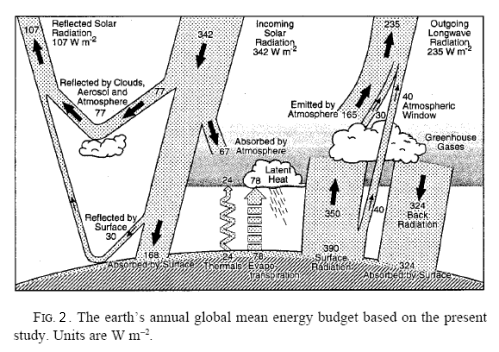
Here is the update in 2009 by Trenberth, Fasullo & Kiehl:

From Trenberth, Fasullo & Kiehl (2009)
Figure 2
The “atmospheric window” value is probably the value in KT97 which has the least attention paid to it in the paper, and the least by climate science. That’s because it isn’t actually used in any calculations of note.
What is the Atmospheric Window?
The “atmospheric window” itself is a term in common use in climate science. The atmosphere is quite opaque to longwave radiation (terrestrial radiation) but the region from 8-12 μm has relatively few absorption lines by “greenhouse” gases. This means that much of the surface radiation emitted in this wavelength region makes it to the top of atmosphere (TOA).
The story is a little more complex for two reasons:
- The 8-12μm region has significant absorption by water vapor due to the water vapor continuum. See Visualizing Atmospheric Radiation – Part Ten – “Back Radiation” for more on both the window and the continuum
- Outside of the 8-12 region there is some transparency in the atmosphere at particular wavelengths
The term in KT97 was not clearly defined, but what we are really interested in is what value of surface emitted radiation is transmitted through to TOA – from any wavelength, regardless of whether it happens to be in the 8-12 μm region.
Calculating the Value
One blog that I visited recently had many commenters whose expectation was that upward emitted radiation by the surface would be exactly equal to the downward emitted radiation by the atmosphere + the “atmospheric window” value.
To illustrate this expectation let’s use the values from figure 2 (the 2009 paper) – note that all of these figures are globally annually averaged:
- Upward radiation from the surface = 396 W/m²
- Downward radiation from the atmosphere (DLR or “back radiation”) = 333 W/m²
- These commenters appear to think the atmospheric window value is probably really 63 W/m² – and thus the surface and lower atmosphere are in a “radiative balance”
This can’t be the case for fairly elementary reasons – but let’s look at that later.
In Visualizing Atmospheric Radiation – Part Two I describe the basics of a MATLAB line by line calculation of radiative transfer in the atmosphere. And Part Five – The Code gives the specifics, including the code.
Running v0.10.4 I used some “standard atmospheres” (examples in Part Twelve – Heating Rates) and calculated the flux from the surface to TOA:
- Tropical – 28 W/m² (52 W/m²)
- Midlatitude summer – 40 W/m² (58 W/m²)
- Midlatitude winter – 59 W/m² (62 W/m²)
- Subarctic summer – 50 W/m² (61 W/m²)
- Subartic winter – 55 W/m² (56 W/m²)
- US Standard 1976 – 65 W/m² (72 W/m²)
These are all clear sky values, and the values in brackets are the values calculated without the continuum absorption to show its effect. Clear skies are, globally annually averaged, about 38% of the sky.
These values are quite a bit lower than the values found in the new paper we discuss in this article, and at this stage I’m not sure why.
This paper is: Outgoing Longwave Radiation due to Directly Transmitted Surface Emission, Costa & Shine (2012):
This short article is intended to be a pedagogical discussion of one component of the KT97 figure [which was not updated in Trenberth et al. (2009)], which is the amount of longwave radiation labeled ‘‘atmospheric window.’’ KT97 estimate this component to be 40 W/m² compared to the total outgoing longwave radiation (OLR) of 235 W/m²; however, KT97 make clear that their estimate is ‘‘somewhat ad hoc’’ rather than the product of detailed calculations. The estimate was based on their calculation of the clear-sky OLR in the 8–12 μm wavelength region of 99 W/m² and an assumption that no such radiation can directly exit the atmosphere from the surface when clouds are present. Taking the observed global-mean cloudiness to be 62%, their value of 40 W/m² follows from rounding 99 x (1 – 0.62).
They comment:
Presumably the reason why KT97, and others, have not explicitly calculated this term is that the methods of vertical integration of the radiative transfer equation in most radiation codes compute the net effect of surface emission and absorption and emission by the atmosphere, rather than each component separately. In the calculations presented here we explicitly calculate the upward irradiance at the top of the atmosphere due to surface emission: we will call this the surface transmitted irradiance (STI).
In other words, the value in the KT97 paper is not needed for any radiative transfer calculations, but let’s try and work out a more accurate value anyway.
First, how the clear sky values vary with latitude:
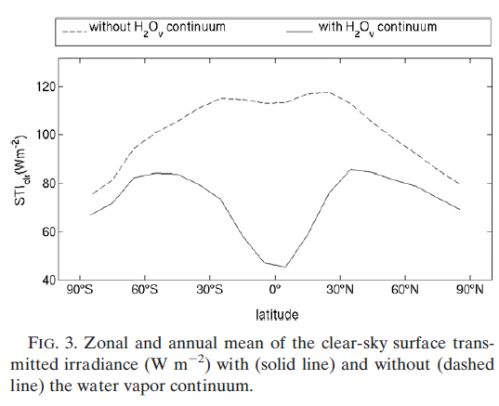
Figure 3 – Clear sky values
Note that the dashed line is “imaginary physics”. The water vapor continuum exists but it is very interesting to see what effect it contributes. This is seen by calculating the effect as if it didn’t exist.
We see that in the tropics STI is very low. This is because the effect of the continuum is dependent on the square of the water vapor concentration, which itself is strongly dependent on the temperature of the atmosphere.
The continuum absorption is so strong in the tropics that STIclr in polar regions (which is only modestly influenced by the continuum) is typically 40% higher than the tropical values.Figure 3 shows the zonal and annual mean of the STIclr to emphasize the role of the continuum. The STIclr neglecting the continuum (dash-dotted line) is generally more than 80 W/m² at all latitudes, with maxima in the northern subtropics (mostly associated with the Sahara desert), but with little latitudinal gradient throughout the tropics and subtropics; the tropical values are reduced by more than 50% when the continuum is included (dashed lines). The effect of the continuum clearly diminishes outside of the tropics and is responsible for only around a 10% reduction in STIclr at high latitudes.
Interestingly, these more detailed calculations yield global-mean values of STIclr of 66 and 100 W/m², with and without the continuum, very close to the values (65 and 99 W/m²) computed using the single global-mean profile, in spite of the potential nonlinearities due to the vapor pressure–squared dependence of the self-continuum.
For people unfamiliar with the issue of non-linearity – if we take an “average climate” and do some calculations on it, the result will usually be different from taking lots of location data, doing the calculations on each, and averaging the results of the calculations. Climate is non-linear. However, in this case, the calculated value of STIclr on an “average climate” does turn out to be similar to the average of STIclr when calculated from climate values in each part of the globe.
We can appreciate a little more about the impact of the continuum on this atmospheric window if we look at the details of the calculation vs wavelength:
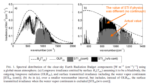
From Costa & Shine (2012)
Figure 4 – Highlighted orange text added
Here is the regional breakdown:
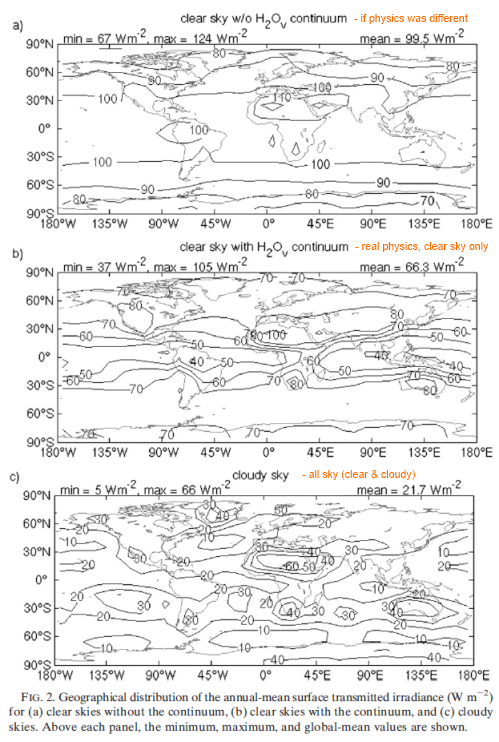
From Costa & Shine (2012)
Figure 5 – Clear and All-sky values – Orange highlighted text added
Note that conventionally in climate science clear sky results are the climate without clouds (i.e., a subset), whereas ‘cloudy sky’ results are the results with both clear and cloudy (i.e., all values).
The authors comment:
When including clouds, the STI is reduced further (Fig. 2c) because clouds absorb strongly throughout the infrared window. In regions of high cloud amount, such as the midlatitude storm tracks, the STI is reduced from a clear-sky value of 70 W/m² to less than 10 W/m². As expected, values are less affected in desert regions. The subtropics are now the main source of the global mean STI. The effect of clouds is to reduce the STI from its clear-sky value of 66 W/m² by two-thirds to a value of about 22 W/m²
Method
They state:
Clear-sky STI (STIclr) is calculated by using the line by line model Reference Forward Model (RFM) version 4.22 (Dudhia 1997) in the wavenumber domain 10–3000 cm-1 (wavelengths 3.33–1000 mm) at a spectral resolution of 0.005 cm-1. The version of RFM used here incorporates the Clough–Kneizys–Davies (CKD) water vapor continuum model (version 2.4); although this has been superseded by the MT-CKD model, the changes in the midinfrared window (see, e.g., Firsov and Chesnokova 2010) are rather small and unlikely to change our estimate by more than 1 W/m²..
..Irradiances are calculated at a spatial resolution of 10° latitude and longitude using a climatology of annual mean profiles of pressure, water vapor, temperature, and cloudiness described in Christidis et al. (1997). Although slightly dated, the global-mean column water amount is within about 1% of more recent climatologies.
Carbon dioxide, methane, and nitrous oxide are assumed to be well mixed with mixing ratios of 365, 1.72, and 0.312 ppmv, respectively. Other greenhouse gases are not considered since their radiative forcing is less than 0.4 W/m² (e.g., Solomon et al. 2007; Schmidt et al. 2010); we have performed an approximate estimate of the effect of 1 ppbv of chlorofluorocarbon 12 (CFC12) (to approximate the sum of all halocarbons in the atmosphere) on the STIclr and the effect is less than 1%.
Likewise, aerosols are not considered. It is the larger mineral dust particles that are more likely to have an impact in this spectral region; estimates of the impact of aerosol on the OLR are typically around 0.5 W/m² (e.g., Schmidt et al. 2010). The impact on the STI will depend on, for example, the height of aerosol layers and the aerosol radiative properties and is likely a larger effect than the CFCs if they are mostly at lower altitudes; this is discussed further in section 4. The surface is assumed to have an emittance of unity.
And later in assumptions:
Our assumption that the surface emits as a blackbody could also be examined, using emerging datasets on the spectral variation of the surface emittance (which can deviate significantly from unity and be as low as 0.75 in the 1000–1200 cm-1 spectral region, in desert regions; e.g., Zhou et al. 2011; Vogel et al. 2011). Some decision would need to made, then, as to whether or not infrared radiation reflected by surfaces with emittances less than zero should be included in the STI term as this reflection partially compensates for the reduced emission. Although locally important, the effect of nonunity emittances on the global-mean STI is likely to be only a few percent.
The point here is that if we consider the places with emissivity less than 1.0 should we calculate the value of flux reaching TOA without absorption from both surface emission AND surface reflection? Or just surface emission? If we include the reflected atmospheric radiation then the result is not so different. This is something I might try to demonstrate in the Visualizing Atmospheric Radiation series.
As is standard in radiative transfer calculations, spherical geometry is taken into consideration via the diffusivity approximation, as outlined in this comment.
Why The Atmosphere and The Surface cannot be Exchanging Equal Amounts of Radiation
This is quite easy to understand. I’ll invent some numbers which are nice round numbers to make it easier.
Let’s say the surface radiates 400 and has an emissivity of 1.0 (implying Ts=289.8 K). The atmosphere has an overall transmissivity of 0.1 (10%). That means 360 is absorbed by the atmosphere and 40 is transmitted to TOA unimpeded. For the radiative balance required/desired by the earlier mentioned commenters the atmosphere must be emitting 360.
Thus, under these fictional conditions, the surface is absorbing 360 from the atmosphere. The atmosphere is absorbing 360 from the surface. Some bloggers are happy.
Now, how does the atmosphere, with a transmissivity of 10%, emit 360? We need to know the atmosphere’s emissivity. For an atmosphere – a gas – energy must be transmitted, absorbed or reflected. Longwave radiation experiences almost no reflection from the atmosphere. So we end up with a nice simple formula:
Transmissivity, t = 100% – absorptivity
Absorptivity, a = 90%.
What is emissivity? It turns out, explained in Planck, Stefan-Boltzmann, Kirchhoff and LTE, that emissivity = absorptivity (for the same wavelength).
Therefore, emissivity of the atmosphere, e = 90%.
So what temperature of the atmosphere, Ta, at an emissivity of 90% will radiate 360? The answer is simple (from the Stefan Boltzmann equation, E=eσTa4, where σ=5.67×10⁻⁸):
Ta = 289.8 K
So, if the atmosphere is exactly the same temperature as the surface then they will exchange equal amounts of radiation. And if not, they won’t. Now the atmosphere is not at one temperature so it makes it a bit harder to work out what the right temperature is. And the full calculation comes from the radiative transfer equations, but the same conclusion is reached with lots of maths – unless the atmosphere is at the same temperature as the surface then they will not exchange equal amounts of radiation.
Conclusion
The authors say:
This study presents what we believe to be the most detailed estimate of the surface contribution to the clear and cloudy-sky OLR. This contribution is called the surface transmitted irradiance (STI). The global- and annual- mean STI is found to be 22 W/m². The purpose of producing the value is mostly pedagogical and is stimulated by the value of 40 W/m² shown on the often-used summary figures produced by KT97 and Trenberth et al. (2009).
Related Articles
References
Earth’s Annual Global Mean Energy Budget, Kiehl & Trenberth, Bulletin of the American Meteorological Society (1997) – free paper
Earth’s Global Energy Budget, Trenberth, Fasullo & Kiehl, Bulletin of the American Meteorological Society (2009) – free paper
Outgoing Longwave Radiation due to Directly Transmitted Surface Emission, Costa & Shine, Journal of the Atmospheric Sciences (2012) – paywall paper


SoD,
If you remember, the whole Eup absorbed equals Edown was a feature of Miskolczi’s theory of the greenhouse effect. A variation of Gresham’s Law, bad money drives out good, seems to apply in the blogosphere, bad theories never go away.
DeWitt,
I remember. This was detailed in The Mystery of Tau – Miskolczi – Part Two – Kirchhoff.
[…] Kiehl & Trenberth and the Atmospheric Window […]
SoD,
One comment on the diffusivity approximation.
The approximation of Zhao and Shi applies perfectly to the calculation of radiation from the surface to space when it’s applied to the full optical depth of the atmosphere. Summing the optical depths without any diffusivity factors and applying Zhao and Shi formula at the end increases transmissivity a little, because doing the correction at the end takes correctly into account the fact that the azimuthal angle stays the same through all layers. (My variation with several theta segments should agree with the corrected version, but it’s not implemented in the same code with standard atmospheres.)
I have added a few lines to the code to allow for correct application of Zhao & Shi formula to this problem. Some changes are observed. For some reason my results don’t fully agree with yours for the uncorrected part, which should be the same. I used dv=1 and CO2 at 360 ppm (my purpose was to have the same value as that of Costa and Shine, but they have 365 ppm)
The results are (atmosphere: corrected value (uncorrected value))
tropical: 34.3 W/m^2 (31.4)
midlatitude summer: 49.2 W/m^2 (46.7)
midlatitude winter: 68.6 W/m^2 (67.2)
subarctic summer: 59.5 W/m^2 (57.5)
subarctic winter: 62.8 W/m^2 (61.4)
US std: 76.0 W/m^2 (74.1)
even without the correction I get significantly (12-15%) higher values than you list in the main article. The results are not particularly sensitive to CO2 concentration as that affects more the radiation from upper troposphere to space. Thus differences in that cannot explain why our results do not agree. The deviations are not so strong that they would change any of the conclusions.
Pekka,
It seems I haven’t really understood this subject. I think I understand your comment above, but I am not sure.
We need to work out emission and absorption for each layer in the atmosphere separately, and to do that we need to know the optical depth τ in each layer.
When we calculate the transmissivity from let’s say 3000m – 4000m we calculate τv (optical thickness for each wavenumber) based first on the number of each absorbing molecule for a thickness of 1000m (and using the density for that layer).
Now this value of τv is only vertically upwards. So we integrate over all solid angles to get the hemispherical absorptivity. I am picturing a thin 1000m shell of atmosphere.
Are you saying that the equation for integrating over all angles is now incorrect (I think this is eqn 6 in Zhao & Shi 2013) ? If yes, for geometrical reasons (because the thin shell is different from a hemisphere)?
My understanding of their formula is that it provides a curve fit to that analytically unsolvable (i.e., only numerically solvable) integration.
If you understand my confusion I’m sure you can explain. It’s possible I have not explained my confusion.
[And in related subjects – I still have to find some time to spend on your implementation of the Voigt line shape].
SoD,
When the question is the transmissivity of a given layer, the whole atmosphere in this case, each azimuthal angle has a pathlength proportional to 1/cos(theta). When the absorptivity is rather high the pathlength affects the transmissivity very strongly and almost all transmission occurs near zenith. When the absorption is very weak all azimuthal angles contribute with equal weight.
The selection based on azimuthal angle starts to occur in the lowest layer. Thus the radiation transmitted trough the first layer is mainly at small theta in case of strong absorption and therefore has a larger probability of passing trough the next layer than it would have without this selection. The effect gets stronger when layers are added.
The above mechanisms is directly simulated in my code that calculates theta segments separately. The Zhao & Shi paper derives the formula that’s valid for a single layer, but does not contain the correlation between successive layers. As it’s correct for a single layer it can be applied to the whole atmosphere when it’s considered as a single layer. It’s easy to add the contributions of each layer in the function optical so that it results in two different outputs:
– single layer tau’s with Zhao & Shi formula applied for each separately
– sum of all layers without Zhao & Shi formula (now I realize that the formula could be applied inside optical, but after summing all layers, but I did that in the main program)
I hope this explanation helps.
I should add that it’s not necessarily true that the Zhao & Shi formula gives better results than the single diffusivity factor 1.66 when it’s applied in a multilayer setting. Reducing the layer thickness brings the constant towards 2.0 with Zhao & Shi and that’s an error. maintaining 1.66 is probably more correct. Thus my guess is that 1.66 is better when numz is large and Zhao & Shi when it’s small, but where the bordering value is that I cannot say.
The only fully correct approach is the multisegment way that works equally and correctly with all numz.
Zhao & Shi is perfect for the whole atmosphere as one layer in the problem of this thread.
SoD,
I keep on wondering why the figures I give in parentheses differ so much from those you present outside parentheses in your post. These numbers should agree as far as I understand.
I do the calculation having nt=3, ocd very large, and tstep very small to prevent changes in temperatures (they all are 0.0). All modifications in molecules, isotopes and concentrations within reasonable limits have much less influence than the difference between our results. I cannot understand, where the difference comes from.
I am a little surprised by the observation that the results for the average atmosphere agree so well with the average of results for varying atmosphere. Although there are obvious factors to reduce the difference, the agreement might be largely accidental and due to the fact that moisture level correlates strongly with surface temperature. Thus the strongest factors just happen to cancel out because of a correlation that’s based on a totally different parts of physics (Clausius-Clapeyron formula, Planck’s law and theory of water vapor continuum are not directly connected).
As the share of direct radiation to space is rather small it’s to be expected that it grows with all kind of variability that applies to conditions where the transmissivity of the atmosphere is relatively high. That applies obviously to dependence on frequency, but that applies also to all spatial and temporal variability. There might be significant effects even from diurnal variability at least when cloudiness is considered.
I am confused about the cloudy sky case. For clear skies most(~80%) of surface radiation in the 8-12μm region reaches the top of the atmosphere. Trenberth calcualtes the average total flux for the IR window in clear skies to be 99 watts/m2. Now lets put a cloud in the way. Photons from the surface are now scattered and absorbed by water droplets at the base of the cloud. However the top of the cloud also emits IR photons as a black body corresponding to the local temperature. Those photons emitted by the top of the cloud in the range 8-12μm continue to escape directly to space. So the top of the cloud now acts exactly like the surface but shifted up in altitude. Therefore a cloud whose ceiling is at say 2000m is to all intents and purposes the same as a surface say in the Alps also at 2000m elevation. In this sense the IR window is still active but merely shifted upwards in altitude. So viewed from space we have one “surface” emitting IR through the window but whose topology is continuously changing. In general though this could can still be considered as some average Earth surface with 60% cloud cover.
What does Trenberth mean by the 30 watts/m2 channel coming out of the cloud ? Is that the IR window component emitted by the tops of clouds ? In that case I would prefer to think of the IR window as being 40+30 = 70 watts/m2. This is because these photons play no role at all in radiative transfer in the rest of the atmosphere.
clivebest,
It’s 99W/m^² through the window for the US 1976 standard atmosphere. But that’s not a good model because the specific humidity is too low.
I’ve never understood the cloud top number either.
Clive,
In essence this is why the STI value is not really a useful value, and has a curiosity value instead. But if we want to know how much of the surface flux is transmitted to the surface without being absorbed then this is the correct calculation.
For your later question, “What does Trenberth mean by the 30 watts/m2 channel coming out of the cloud?” – which reference are you talking about?
There is a value called “cloud radiative forcing” which is usually worked out as a longwave and shortwave component. The cloud longwave radiative forcing is about 30 W/m2 – this is the reduction in OLR as a result of clouds. If I have the right value that you are asking about and it doesn’t make sense I can try and explain a little further and also dig up a reference.
SoD,
What I’m, and I think clivebest, are talking about is the arrow or path in the cartoon next to the ‘Emitted by Atmosphere’ arrow labeled 30 that appears to originate from a cloud top. That number has never made any sense to me. I don’t see how that has anything do do with radiative forcing by clouds as that would lead to a reduction in emission.
30 W/m^2 directly transmitted from the cloud tops to space seems much too low to me, as there is very little water vapor above the clouds.
I think the diagram, without the commentary, is confusing for this part.
KT97 say, in reference to this figure:
If we go back earlier in the paper the longwave cloud forcing is explained. It’s not the most intuitive of subjects..
The OLR for clear skies is 30 W/m2 more than the OLR for all-skies.
By convention, clear skies are a subset, and cloudy skies refers to all skies.
So to answer specifically RW’s question, if it’s not already clear, the emission of longwave radiation from clouds is much higher than 30 W/m2. This value is defined as how much the TOA flux changes between clear skies and cloudy (all) skies.
SoD.
“In essence this is why the STI value is not really a useful value, and has a curiosity value instead.”
You are right in the sense that a line by line radiative transfer calculation like yours doesn’t need this value – it is a result of the calculation. However I still think STI is an important feature of the Earth’s energy balance compared to say that on Venus. The Costa & Shine paper show how strongly this varies with humidity in the tropics, and that overall Trenberth’s numbers are likely too high. However as far as I understand it Trenberth’s “estimate is based on the following
Clear sky standard atmosphere IRW(STI) = 99 watts/m2
Average cloud cover = 60% -> average IRW originating from surface = 40 watts/m2
So on average 60 watts/m2 emitted directly from the surface in the IR window is absorbed by clouds. Clouds are droplets of liquid water – not water vapour. In that sense they are more like the oceans and radiate as a diffuse black body. They radiate IR over the full BB spectrum not just in the water continuum/lines. So the tops of clouds radiate at all wavelengths just like the surface – it is just that they are colder. Water vapour and CO2 lying above the clouds then absorb/thermalize ~70% of it leaving a “cloud sourced IR” window to radiate to space.
Lets just guess that the average temperature of tops of clouds is 273K. BB radiation emitted by clouds is then roughly 0.8 times that of the surface and globally there is about an average of 0.6 cloud cover. So I estimate that clouds radiate ~0.5 times that from the surface. Overall then
Clear skies = 0.4
Cloudy skies = 0.5
Total = 0.9
So clouds block ~10% of surface radiation . This is fairly close to 30 watts/m2. This value is what I (perhaps mistakenly) interpret as the statement made above :
However clouds tops must also radiate through the IR window. That fraction of the IR spectrum in the window is roughly going to be (0.8 x 0.6)*99 = 47 watts/m2.
These figures may well be wrong, but I do think that the tops of clouds radiate directly to space through the IR window as shown in the Trenberth cartoon.
Clive
I agree with you, which is why I have posted articles on % of flux transmitted from the surface to TOA, % of flux from each height contributing to TOA, what the atmospheric radiation would look like without atmospheric emission, etc.
So in essence it is a useful value to understand how climate works. And perhaps I am being unclear/unfair in painting it as a “curiosity value”. What I mean is, its correctness or otherwise isn’t necessary for climate models. But it is very useful for understanding.
I think your calculation of the various fractions is not correct, even though some of the reasoning is correct.
It’s not as simple as:
Unless you can write down something more complete? Clear skies = 0.4 of what? If we are talking about TOA:
TOA = clear sky TOA + LWCF
TOA = cloudy sky TOA (because cloudy sky = all sky)
Alternatively, if we are talking about the atmospheric window your values are more correct, but as Costa & Shine have shown, the window is not a window in the humid tropics.
The reason clouds have a change in OLR in contrast to clear skies is for the answer you gave. Then there are clouds of different heights. Low clouds have pretty much the same OLR as the surface, so not much (longwave) effect – but they do have a big shortwave effect (reflecting much more solar). High clouds have a much different OLR compared with the surface so they have a large (longwave) effect.
Hopefully this is clear.
Sorry for not being clear. What I meant was fraction of the surface radiation (Is) reaching TOA under clear skies for a surface temperature Ts=288K. If we arbitrarily define the average temperature of the tops of clouds to be Tc=273K. Then we have for top of cloud radiation Ic
Ic/Is = (273^4)/(288^4) = 0.8
So if 40% of the Earth’s surface has clear skies and 60% has cloud covered skies then very approximately we have
I(net) = 0.4Is +0.6(0.8Is)
~ 0.9Is –> clouds reduce total surface radiation by ~10%
Now following Trenberth – about 25% of Is (99/390) passes through the IR window in clear skies. Likewise we simply assume that 25% of Ic also passes through the IR window -so finally:
I(IRW) = 0.4*99 + 0.6*(0.8*99) = 0.88*99 = 87 watts/m2
These numbers are not intended to be taken too seriously !
SoD,
That’s reasonable. In fact if you run MODTRAN with cloud covered sky, that’s close to the reduction in OLR that’s observed.
Indeed. The diagram makes it look like there is more emission from clouds, not less. It should have 30 W/m² of atmospheric emission disappearing into the cloud, not apparently being emitted from the cloud top.
DeWitt,
I agree. The table contains values 265 for clear sky TOA and 235 for cloudy sky TOA. Thus the clouds act here as a sink, not as a source.
Pekka, Dewitt,
I can’t agree that it is simply that 30 W/m2 is lost into clouds rather than emitted from the top of clouds.
Look again at Figure 7. Kiehl & Trenberth 1997. The outgoing 235 watts/m2 is for the globally averaged “cloudy” case. The 30 watts/m2 is actually added to that emitted only by greenhouse gases (165 watts/m2). This must be some average between clear skies (265 watts/m2) and 100% cloud cover (X watts/m2). Assuming that the surface IR window remains constant, we can find X by using:
235 = 0.4*265 + 0.6*X
X = 215 w/m2
now subtracting a fixed IR window of 40 w/m2 from both sides
195 = 0.4*225 +0.6*X
so X = 175 watts/m2
I think instead it is more like 60 w/m2 is taken out by clouds but then 30 w/m2 is returned from the cloud tops !
I am open to correction of course !
The 1997 paper states explicitly that the number 30 represents LWFC. It explains also that LWFC is the reduction of OLR at TOA from 265 to 235. That’s all very explicit.
The graphics show at the top 235 and 40 as part of that leaving 205 for the rest, but nothing in the paper is 205 (the 205 is shown as 165+40).
The graphics presents numbers that do not correspond to anything in the paper and is explicitly in contradiction with a reasonable interpretation of the text.
All this is confusing and shows lack of care in drawing the graphics. Otherwise it’s inconsequential.
I don’t think clouds are inconsequential. Rather I think clouds and water vapour stabilize the climate. I have been studying the NASA NVAP data and water vapour in the upper atmosphere has clearly decreased since 1988 while CO2 has increased.
Clouds are certainly important, but considered also self-evident that the graphics has so little on clouds that it cannot be considered a source for understanding the effects of clouds.
This is what Trenberth says in this paper. http://www.cgd.ucar.edu/cas/Trenberth/trenberth.papers/QJRMSenergyflow04.pdf
So I think it is just a coincidence that the net radiative forcing of clouds = 30 watts = radiation to space from top of clouds.
Clive,
Check again what the paper says about this particular number:
The paper doesn’t leave freedom to interpret that in any other way than SoD and I have written.
I accept that is what KT97 says and SoD’s interpretation as well. Let me try one last time to explain why I think the cartoon in the paper is still correct to show cloud tops radiating 30 watts.
Quoting from the main post by SoD above on STI.
1. KT97 finds STI to be. Clear Skies=99 and Cloudy Skies=40
2. KT97 finds OLR at TOA to be. Clear Skies= 265 and Cloudy Skies = 235
From 2: LWCF = 30 W/m2
From 1: STI absorbed by clouds = 59 W/m2
Therefore 29 W/m2 radiates from the top of clouds through the IR window to space to balance energy ! 59=30+29. This is what the cartoon really shows IMHO.
P.S. I am trying to type this on an IPAD and which has the annoying habit of auto-correction so I hope the blockquote above works !
clivebest,
That may all work out mathematically, but physically it makes no sense at all, which is why it’s confusing. Little or no surface radiation actually penetrates a cloud covered sky. In MODTRAN, the average transmittance from 100-1500 cm-1 for a cloud is 0.0000. OTOH, the window at the altitude of cloud tops is huge. For MODTRAN with the 1976 US standard atmosphere with cumulus cloud cover base 0.66km, top 2.7km at a viewing height of 3.5km looking down we get 272.112 W/m² emission from 100-1500 cm-1. In spite of it saying that the cloud top is 2.7 km, you’re still inside the cloud until you set the observation altitude at 3.5 km. The average transmittance to space at that altitude is 0.4149. So 112.9 W/m² is transmitted directly to space from the cloud top, not 30 W/m². That’s for low level clouds. The window just gets bigger for higher level clouds while the emission gets smaller.
“Little or no surface radiation actually penetrates a cloud covered sky. ”
Correct – so 60 W/m2 of surface radiation in the 8-12um region is absorbed immediately by the base of the cloud. The top of the cloud though is at a much lower temperature and emits as a black body something like ~100 W/m2. Most of this is thermalised (or radiatively transferred) by greenhouse gases above the cloud. BUT there is still about 30 W/m2 of the BB spectrum which lies within the 8-12um region that passes straight through to space.
I didn’t correct for surface coverage. If we assume 60% cloud cover and ignore mid and high level clouds, the 30W/m² from cloud tops to space should be increased to 68W/m² and emitted by atmosphere reduced to 131W/m². That would be physically realistic.
DeWitt,
I agree. I just add an additional point.
We can have so much radiation from the clouds to space, because in absence of the clouds we have much radiation from the water vapor of low atmosphere to space and clouds block that in addition to blocking the radiation from the surface. Here the moisture profile of the atmosphere plays a major role.
I answered too quickly to Dewitt. I think we are almost in agreement. On a global average, cloud tops emit X w/m2 directly to space where X is 30 w/m2 less than that emitted by 100% clear skies. Figure 2 in KT97 is misleading in so far as it assigns X as 30 W/m2.
I had a look at the calculations that I made with SoD’s model for the standard atmospheres. Taking as example the midlatitude summer, about 90 % of the optical depth in the region of the atmospheric window is from the lowest 3 km. Thus the radiation from the altitudes below 3 km is a very important part of the radiation from atmosphere to space over the range 700-1300 1/cm. There’s some additional effect from wavenumbers 400-650 1/cm and 2000-2300 1/cm.
SoD says;
“As a result of this changed value, of course the standard energy balance diagram shown in KT97 and TFK09 needs some adjustments.”
There is a serious problem here if the ‘window’ average value is changed.
If we examine all the other average values in TFK09 they are all given to an accuracy of three significant figures.
So if they are to be changed then then this level of claimed accuracy is a fraud.
Just fiddling around with the numbers to obtain a new set of averages that satisfies the first law as far as solar input and IR output are concerned will be looked on as pseudoscience.
The more reckless IPCC advocates might question whether the first law applies to heat transfer if to radiative transfer is involved.
They don’t claim this level of accuracy as anyone reading the paper through can grasp.
Phrases like:
“..However, there is considerable uncertainty in precipitation over both the oceans and land (Trenberth et al. 2007b; Schlosser and Houser 2007)..”
“..TOA values are known within about ±3% or better..”
and the plain English of the paper makes is a useful document for anyone trying to understand the global TOA and surface energy balance – and the relative uncertainties.
And in KT97 they say:
Of course, Bryan has demonstrated his unhappiness with KT97 and TFK09. It’s good to see he still hasn’t read the paper.
SoD
It appears that the given ‘window’ value of 40W/m2 might be as high as 62W/m2.
In any of the ‘hard’ sciences this value would be written as 5×10^1 ±20%
If Climate Science hopes to be taken seriously it must comply with these accepted standards.
When the real uncertainties are included in the KT97 and TFK09 diagrams its hard to justify the alarmist viewpoint.
The direct effect of a doubling of atmospheric CO2 is said to be in the order of 1W/m2.
Its clear that this value is swamped by the uncertainties in the other values.
SoD says
” Regardless of the errors assigned to each component,the fact that the components sum to zero means some errors must cancel.”
The assumption that errors must cross cancel is unwarranted.
If this then leads to assigning convenient values to achieve this result, then you will be trapped in a circular logic loop.
Curiosity values are only that. It’s not relevant for anything else. Therefore the limits of uncertainty matter little and the value is given as an illustrative one without claims on accuracy.
Bryan says:
Only if you can’t read what the paper says. Which I quite believe. In fact, I’m certain of it.
Bryan previously said:
Whereas the paper said something different.
In summary, we can confirm that your only issue with KT97 is that you don’t believe it follows a convention on stating uncertainty?
So your working position is that finally, you have grasped what the authors have been saying since 1997 (and they follow a long list of atmospheric physicists who have also tried to work out the various values and uncertainties) and based on that, now say:
Correct?
Your genius is most likely in convincing people that there is much less likely to be something in what might be misleadingly entitled “the skeptic position”.
And also you believe that even though an accurate assessment can be made of the change in net absorption by the climate system due to increases in GHG’s, because surface energy balance components are not known to the same degree of accuracy, therefore, this change in net absorption must vanish somewhere?
I don’t expect a sensible response. You do the world of climate science a huge favor by illustrating… [moderator’s note – deleted due to breach of blog etiquette]
SoD
At the start of this post you said
“One blog that I visited recently”
I take it that you were referring to the Tallbloke site ( it would have helped if you had given a link).
In turn the Tallbloke discussion linked back to your own site.
In replies Christopher Game disclosed that Trenberth now agrees that the given ‘window’ value of 40W/m2 might be as high as 62W/m2.
If true this is a startling admission.
Your site is full of claims that the figures given in the KT97 and TFK09 diagrams are ‘hard’ numbers independently experimentally confirmed.
For instance the ‘backradiation’ figure of 333W/m2 implies a resolution to the last ± one watt/m2.
That’s the convention in normal science but apparently not in climate science.
SoD says
“In summary, we can confirm that your only issue with KT97 is that you don’t believe it follows a convention on stating uncertainty?”
You certainly cannot draw this conclusion.
These diagrams are full of errors.
It will be interesting to see which of the values are candidates for ‘adjustment’.
[…] 2013/02/02: TSoD: Kiehl & Trenberth and the Atmospheric Window […]
[…] 2013/02/02: TSoD: Kiehl & Trenberth and the Atmospheric Window […]
[…] the 800-1200 cm-1 region (8-12 μm), the so-called “atmospheric window” – see Kiehl & Trenberth and the Atmospheric Window. We will come back to the reasons why in a […]
I have read this article and all blogs with care, but what i am missing in all calculations or comments are round about 80 W/m² sw radiation absorpted in atmosphere and 100 W /m² going up from surface to atmosphere in form of latent and convectiv heat. Part of this extra flux has also to go to space in form of lw radiation and must be on final part of OLR.
Not only 396 W/m² are going from ground to atmosphere, If we take the K&T 09 numbers, we have to add 97 W/m² to the upgoing flux and we have not to worry about, wether it is radiation or matter-bounden energy, because on final it must be changed all to radiation in order to leave to space.
Taking tau=1,867 from Miskolczi you get the amount of 61,4 W/m² STi, looks pretty good like USS76 Value.
correct?
This article is specifically about this one point of the much-discussed “Atmospheric window”.
What’s the Palaver? – Kiehl and Trenberth 1997 covered more of the overall picture.
I don’t understand your question. Can you clarify?
The paper doesn’t explain the first law of thermodynamics, it just assumes readers understand it.
The surface is in approximate energy balance; which means energy in = energy out.
Solar absorbed + longwave absorbed = longwave radiated + convected
-Using KT97 numbers for convenience: 168 + 324 = 390 + 102 = 492 [tick]
The climate system as a whole is in approximate energy balance:
Solar absorbed by surface + solar absorbed by atmosphere = longwave emitted by the whole climate system
168 + 77 = 235 [tick]
KT97 uses the first law of thermodynamics to calculate the items most difficult to ascertain from measurements – as a balancing item.
You can see more about Miskolczi in this series.
[…] Kiehl & Trenberth and the Atmospheric Window […]
Kiehl & Trenberth 1997 says the following:
I guess no one ever learned how to do interpolation. If the clear sky case is 99 W/m^2 and the cloudy sky case is 80 W/m^2, then the 62% cloudy/38% clear interpolation should give you about 87 W/m^2. Instead, they are interpolating between 99 W/m^2 and 0 W/m^2 (38% of the clear sky case). They can’t even do that right, as it should be slightly less than 38 W/m^2–not 40 W/m^2.
Why is 40 W/m^2 the answer?
Jim
Jim: 40 W/m2 is K&T estimate for the power in the LWR photons with “window wavelengths” that are emitted directly from the surface to space through clear skies. This number is shown on the K&T diagram.
LWR photons with “window wavelengths” are also emitted to space from cloudy skies. Those photons obviously come from clouds, not the surface. (Unlike the GHGs in clear skies, clouds emit and absorb a blackbody spectrum and some fall within “window wavelengths”.)
If the K&T diagram showed us how much power is escaping to space at “window wavelengths”, your answer of 87 W/m2 would be the correct one. But they are illustrating only the direct flux from surface to space that has not modified by the atmosphere (GHGs or clouds).
KT97 is assuming 62% cloudiness. I’m saying the number 40W/m^2 is wrong based on the statements made in the paper. I know what the diagram shows. They also say it’s 99 W/m^2 for a clear sky. So your comment doesn’t follow.
Jim
Jim: Does saying that “the average m^2 of surface emits 99 W/m2 to space the 40% of the time it is clear overhead” work for you? And 0 W/m2 DIRECTLY TO SPACE when it is cloudy? That is an average of 40 W/m2 directly to space.
What works for me is doing the math correctly. When they say that it’s 80 W/m^2 for the cloudy case, that’s not 0 W/m^2–far from it. And when they say 38% of 99 W/m^2 is 40 W/m^2 instead of (less than) 38 W/m^2, they are playing with numbers.
So why the hand-wringing about a missing 0.5 W/m^2 when they are rounding by more than 2 W/m^2?
Jim
Jim,
I’m sure I’m wasting my time here, but try looking at the diagram again. The 40 W/m² is coming directly from the surface, averaged over the entire surface. ALL the rest of the surface radiation is absorbed by the atmosphere and clouds. The 80W/m² emitted by cloud tops has exactly nothing whatsoever to do with the 40W/m² emitted from the surface directly to space.
Oh, and not all the radiation that escapes directly to space is in the ‘window’. That’s why the total is 40W/m² and not 37.6W/m².
I just don’t see how it can be so hard to read what the paper is saying instead of making things up!
They ARE talking about radiation in the “window.” They aren’t interpolating correctly, and I don’t know what math you’re using Mr. Payne.
Jim
Jim Masterson,
DeWitt is using simple, clear math. With no clouds, there would be 99 W/m^2 emitted from the surface in the window. With 42% clear sky, there is 38 W/m^2 emitted in the window from the surface, plus 42 W/m^2 emitted by clouds in the window, for a total of 80 W/m^2 in the window. Since the clouds absorb in the window region, they must also emit in the window. And since the clouds are cooler than the surface, they emit less than the surface would have. I am assuming that you have cited the numbers correctly.
Jim,
Are you incapable of understanding that the source of radiation to space means something and matters? Apparently.
I was correct, it was a waste of time engaging you. Bye.
I found this article again, and the picture can be studied in many ways comparing the various contributions. I wonder how the non LW energi to the atmosphere (78+17+80=175) is split between up and down LW radiation.
Is there any papers that try to make a closer accounting for the LW part of the radiation including the 175W that is delivered as heat to the atmosphere and then converted to radiation going up and down.
Svend,
Energy is fungible. It’s impossible to track individual joules in a system. So asking how a specific fraction, say non LW, of energy to the atmosphere is split between up and down has no answer other than it’s the same fraction as the total energy. Needless to say, there are no papers that try to make a closer accounting.
Svend: One way to express the “fungibility” of energy is to simply add up all of the fluxes between various compartments, say BETWEEN the surface and the atmosphere: -396+333-17-80 = -180. W/m2 as a single arrow. The net flux, ie heat, is flowing from the generally warmer surface to the generally cooler atmosphere.
And you should be aware that all fluxes are two-way fluxes, but only LWR is shown that way. For example, the evaporation of water shown in this figure is the net result of a two-way processes. Over the ocean (where relative humidity is about 80%), the downward flux of latent heat in water molecules traveling directly from the atmosphere to the ocean is 80% size of the upward flux. If the net flux were the 80 W/m2 shown in this figure, there would be 400 W/m2 of latent heat in the water molecules evaporating and 320 W/m2 in the water vapor returning directly to the surface (ie not as rain). We know this because the rate of net evaporation depends on relative humidity of the air above the water and goes to zero when that air is saturated.
Thermodynamics originated with the study of heat engines, where the two-way fluxes occur on too small a scale to be observed. Today we know that slower-moving molecules frequently collide with and transfer kinetic energy to faster-moving molecules – though transfer in the opposite direction is more common. Temperature is the concept we developed to keep track of the average kinetic energy of a group of many rapidly colliding molecules and heat is the concept we use to track the net flux of energy between two groups of molecules.
For consistency, the above energy balance diagram “should” show only the net LWR flux from the surface to the atmosphere, or show evaporation of water as a two-way flux, SWR arriving at the surface as a two-way flux (with a negligible amount of visible light being emitted by the surface), and sensible heat as a two-way flux, etc. All are two way processes. The thing that differentiates radiation from all of these other energy fluxes is that photons travel long distances compared with molecules and we can easily measure the flux of photons in both directions. Because the flux of LWR is the only one explicitly shown as a two-way flux, conspiracy theorists have developed all sorts of strange ideas.
I understand it is hard or impossible to split the non-LW radiation. I believe anyway that this heat could be dilivered in diffent parts of the atmospher, where the latent heat and convection mostly is influencing the lower part and the absorbed SW could be delivered in the upper part.
Besides that i find the back radiation (333) quite large. Is it possible to split it between radiation from clouds and radiation from the atmospheres GHG’s.?
It was a too quick asking. I checked the Surfrad and found that the back radiation varies less than 100W between cloud and clear sky,This small difference makes it impossible to split the back radiation between the sources.
Nevertheless is there any plots of back radiation spectrum?
There is a lot of plots for the radiation to space, but i have never seen the same for the back radiation.
I know the picture K&T gives is an overall picture like a koncern balance, All the subdivisons and there contributions and internal trading is hidden.We can only make som educated guesses of the balance and trading for the subdiviaions.
Svend,
You can see plots of back radiation measured at the surface here:
The Amazing Case of “Back Radiation” – Part Two.
It’s definitely possible to calculate the split between clouds and the clear sky atmosphere. However, it requires details of the global state at a given time – for cloudy areas cloud height, thickness plus water vapor profile below at each point around the globe + for non-cloudy sky the water vapor profile at each point around the globe (depending on the resolution you want in your answer).
If you wanted to calculate the split over a year or a decade then you would need to decide on a time step and get the data for each time step, do the calculation, then average over the whole time period.
For probably everyone in climate science it’s not an interesting calculation, it’s a curiosity.
Svend: You can also use Modtran to predict DLR for various idealized situations: For example, you can compare DLR during midlatitude summer (high humidity) and winter (low humidity) with or without clouds at various altitudes. The average photon arriving at the surface is emitted from a lower altitude in summer than winter, because some have wavelengths capable of being absorbed and emitted by water vapor. In winter in the midlatitudes, at the “atmospheric window” wavelengths, you can “see” all the way to space, and space emits no energy these wavelengths. This isn’t true in summer. You can remove water vapor from the atmosphere by entering 0 on the water vapor scale and find that it is responsible for obscuring infrared in the “atmospheric window”. (Or better still, you can look at the DLR emission from a one GHG at a time before making guessed about the complicated spectrum of DLR from the real atmosphere.)
All clouds with low bases deliver DLR with a blackbody spectrum and intensity appropriate for the temperature at their base. The DLR arriving at the surface below higher altostratus clouds is significantly modified by absorption and emission on its way to the surface.
Real observations of DLR in other posts linked by SOD complement what radiation transfer calculations predict for certain idealized atmospheric models like “midlatitude summer” or “US Standard Atmosphere”. However, whenever scientists go into the field and compare observations of the spectrum and intensity of DLR with predictions made by radiation transfer calculations, the agreement is good. (To makes calculations in the field, you need temperature and humidity data at all altitudes from a radiosonde launched at the observing site.) Apparently there are minor difficulties due to aggregation of water vapor molecules at high humidity (the “water vapor continuum”) only near the surface. For most other situations, the accuracy of the calculations is comparable to the accuracy of the instruments used to measure IR in the field.
I really enjoy conducting “experiments” with Modtran to answer questions like yours, but in the end there is always the frustration that the answer you get is for one or a few idealized atmospheric models and not a “global” value. However, even the best AOGCMs disagree about global values for DLR and have been tuned to make OLR and OSR agree with imperfect measurements made by satellites.
http://climatemodels.uchicago.edu/modtran/
Thanks for the explanations and answers.
One important lesson i have learned is, that the net LW radiation from Earth to TOA can increase if there are other heatsources than the LW radiation from Earth. Here the heat sources are solar absorbtion, convection and latent heat.
-Svend