In an earlier article on water vapor we saw that changing water vapor in the upper troposphere has a disproportionate effect on outgoing longwave radiation (OLR). Here is one example from Spencer & Braswell 1997:
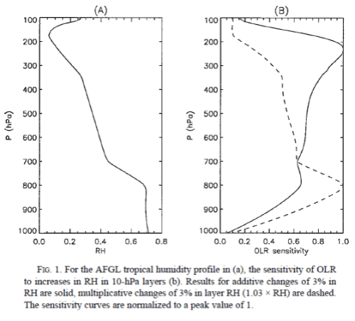
From Spencer & Braswell (1997)
Figure 1
The upper troposphere is very dry, and so the mass of water vapor we need to change OLR by a given W/m² is small by comparison with the mass of water vapor we need to effect the same change in or near the boundary layer (i.e., near to the earth’s surface). See also Visualizing Atmospheric Radiation – Part Four – Water Vapor.
This means that when we are interested in climate feedback and how water vapor concentration changes with surface temperature changes, we are primarily interested in the changes in upper tropospheric water vapor (UTWV).
Upper Tropospheric Water Vapor
A major problem with analyzing UTWV is that most historic measurements are poor for this region. The upper troposphere is very cold and very dry – two issues that cause significant problems for radiosondes.
The atmospheric infrared sounder (AIRS) was launched in 2002 on the Aqua satellite and this instrument is able to measure temperature and water vapor with vertical resolution similar to that obtained from radiosondes. At the same time, because it is on a satellite we get the global coverage that is not available with radiosondes and the ability to measure the very cold, very dry upper tropospheric atmosphere.
Gettelman & Fu (2008) focused on the tropics and analysed the relationship (covariance) between surface temperature and UTWV from AIRS over 2002-2007, and then compared this with the results of the CAM climate model using prescribed (actual) surface temperature from 2001-2004 (note 1):
This study will build upon previous estimates of the water vapor feedback, by focusing on the observed response of upper-tropospheric temperature and humidity (specific and relative humidity) to changes in surface temperatures, particularly ocean temperatures. Similar efforts have been performed before (see below), but this study will use new high vertical resolution satellite measurements and compare them to an atmospheric general circulation model (GCM) at similar resolution.
The water vapor feedback arises largely from the tropics where there is a nearly moist adiabatic profile. If the profile stays moist adiabatic in response to surface temperature changes, and if the relative humidity (RH) is unchanged because of the supply of moisture from the oceans and deep convection to the upper troposphere, then the upper-tropospheric specific humidity will increase.
[Emphasis added]
They describe the objective:
The goal of this work is a better understanding of specific feedback processes using better statistics and vertical resolution than has been possible before. We will compare satellite data over a short (4.5 yr) time record to a climate model at similar space and time resolution and examine the robustness of results with several model simulations. The hypothesis we seek to test is whether water vapor in the model responds to changes in surface temperatures in a manner similar to the observations. This can be viewed as a necessary but not sufficient condition for the model to reproduce the upper-tropospheric water vapor feedback caused by external forcings such as anthropogenic greenhouse gas emissions.
[Emphasis added].
The results are for relative humidity (RH) on the left and absolute humidity on the right:
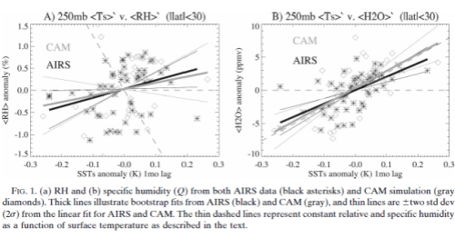
From Gettelman & Fu (2008)
Figure 2
The graphs show that change in 250 mbar RH with temperature is statistically indistinguishable from zero. For those not familiar with the basics, if RH stays constant with rising temperature it is the same as increasing “specific humidity” – which means an increased mixing ratio of water vapor in the atmosphere. And we see this is the right hand graph.
Figure 1a has considerable scatter, but in general, there is little significant change of 250-hPa relative humidity anomalies with anomalies in the previous month’s surface temperature. The slope is not significantly different than zero in either AIRS observations (1.9 ± 1.9% RH/°C) or CAM (1.4 ± 2.8% RH/°C).
The situation for specific humidity in Fig. 1b indicates less scatter, and is a more fundamental measurement from AIRS (which retrieves specific humidity and temperature separately). In Fig. 1b, it is clear that 250- hPa specific humidity increases with increasing averaged surface temperature in both AIRS observations and CAM simulations. At 250 hPa this slope is 20 ± 8 ppmv/°C for AIRS and 26 ± 11 ppmv/°C for CAM. This is nearly 20% of background specific humidity per degree Celsius at 250 hPa.
The observations and simulations indicate that specific humidity increases with surface temperatures (Fig. 1b). The increase is nearly identical to that required to maintain constant relative humidity (the sloping dashed line in Fig. 1b) for changes in upper-tropospheric temperature. There is some uncertainty in this constant RH line, since it depends on calculations of saturation vapor mixing ratio that are nonlinear, and the temperature used is a layer (200–250 hPa) average.
The graphs below show the change in each variable as surface temperature is altered as a function of pressure (height). The black line is the measurement (AIRS).
So the right side graph shows that, from AIRS data of 4 years, specific humidity increases with surface temperature in the upper troposphere:
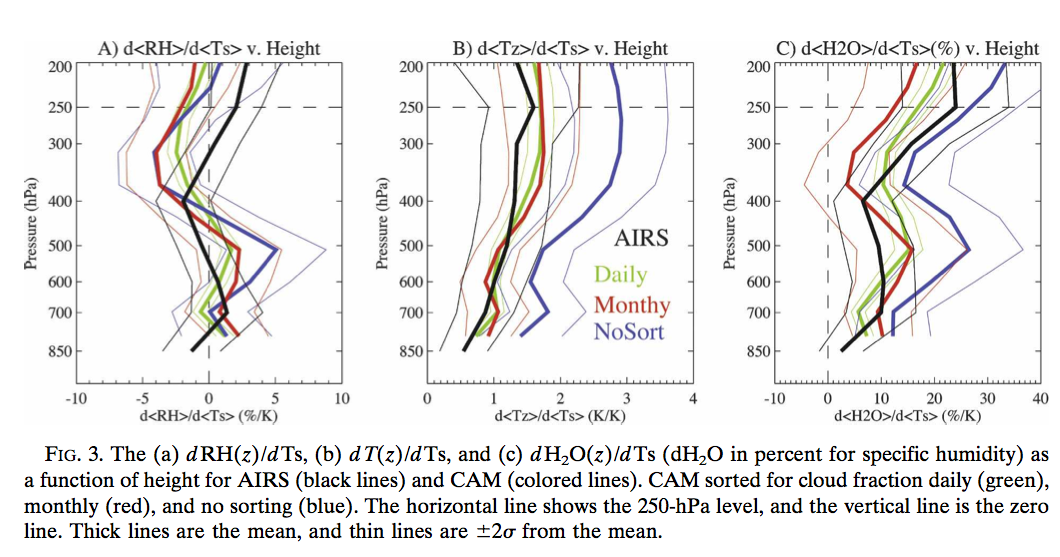
From Gettelman & Fu (2008)
Figure 3 – Click to Enlarge
There are a number of model runs using CAM with different constraints. This is a common theme in climate science – researchers attempting to find out what part of the physics (at least as far as the climate model can reproduce it) contributes the most or least to a given effect. The paper has no paywall, so readers are recommended to review the whole paper.
Conclusion
The question of how water vapor responds to increasing surface temperature is a critical one in climate research. The fundamentals are discussed in earlier articles, especially Clouds and Water Vapor – Part Two – and much better explained in the freely available paper Water Vapor Feedback and Global Warming, Held and Soden (2000).
One of the key points is that the response of water vapor in the planetary boundary layer (the bottom layer of the atmosphere) is a lot easier to understand than the response in the “free troposphere”. But how water vapor changes in the free troposphere is the important question. And the water vapor concentration in the free troposphere is dependent on the global circulation, making it dependent on the massive complexity of atmospheric dynamics.
Gettelman and Fu attempt to answer this question for the first half decade’s worth of quality satellite observation and they find a result that is similar to that produced by GCMs.
Many people outside of climate science believe that GCMs have “positive feedback” or “constant relative humidity” programmed in. Delving into a climate model is a technical task, but the details are freely available – e.g., Description of the NCAR Community Atmosphere Model (CAM 3.0), W.D. Collins (2004). It’s clear to me that relative humidity is not prescribed in climate models – both from the equations used and from the results that are produced in many papers. And people like the great Isaac Held, a veteran of climate modeling and atmospheric dynamics, also state the same. So, readers who believe otherwise – come forward with evidence.
Still, that’s a different story from acknowledging that climate models attempt to calculate humidity from some kind of physics but believing that these climate models get it wrong. That is of course very possible.
At least from this paper we can see that over this short time period, not subject to strong ENSO fluctuations or significant climate change, the satellite date shows upper tropospheric humidity increasing with surface temperature. And the CAM model produces similar results.
Articles in this Series
Articles in the Series
Part One – introducing some ideas from Ramanathan from ERBE 1985 – 1989 results
Part One – Responses – answering some questions about Part One
Part Two – some introductory ideas about water vapor including measurements
Part Three – effects of water vapor at different heights (non-linearity issues), problems of the 3d motion of air in the water vapor problem and some calculations over a few decades
Part Four – discussion and results of a paper by Dessler et al using the latest AIRS and CERES data to calculate current atmospheric and water vapor feedback vs height and surface temperature
Part Five – Back of the envelope calcs from Pierrehumbert – focusing on a 1995 paper by Pierrehumbert to show some basics about circulation within the tropics and how the drier subsiding regions of the circulation contribute to cooling the tropics
Part Six – Nonlinearity and Dry Atmospheres – demonstrating that different distributions of water vapor yet with the same mean can result in different radiation to space, and how this is important for drier regions like the sub-tropics
Part Seven – Upper Tropospheric Models & Measurement – recent measurements from AIRS showing upper tropospheric water vapor increases with surface temperature
Part Eight – Clear Sky Comparison of Models with ERBE and CERES – a paper from Chung et al (2010) showing clear sky OLR vs temperature vs models for a number of cases
Part Nine – Data I – Ts vs OLR – data from CERES on OLR compared with surface temperature from NCAR – and what we determine
Part Ten – Data II – Ts vs OLR – more on the data
References
Observed and Simulated Upper-Tropospheric Water Vapor Feedback, Gettelman & Fu, Journal of Climate (2008) – free paper
How Dry is the Tropical Free Troposphere? Implications for Global Warming Theory, Spencer & Braswell, Bulletin of the American Meteorological Society (1997) – free paper
Notes
Note 1 – The authors note: “..Model SSTs may be slightly different from the data, but represent a partially overlapping period..”
I asked Andrew Gettelman why the model was run for a different time period than the observations and he said that the data (in the form needed for running CAM) was not available at that time.


That’s really ugly data. The RH plot looks like a shotgun pattern and the specific humidity plot doesn’t look much better. I should look at the paper and see what sort of statistical tests they used to determine significance. Serial autocorrelation, for example, would widen the confidence limits because it reduces the effective degrees of freedom.
It seems to be the way with measuring the real climate – the data is ugly.
I did ask how sensitive the data was to outliers and the response from Andrew Gettelman: “..The bootstrap method randomly samples the data to generate a distribution from which the uncertainty on the fit can be assessed: precisely why I used it in this case..”
I’m novice level on stats so find it difficult to assess any statistics.
I haven’t looked at these issues very much, but my first impression is that reading first the 2006 paper Climatology of Upper-Tropospheric Relative Humidity from the Atmospheric Infrared Sounder and Implications for Climate of Gettelman et al is very helpful.
This later paper discusses changes in humidity, but does not tell about the actual levels. In the 2006 paper we find information on that, again both from AIRS and from CAM simulations. There we see that the model agrees reasonably well with the data, but that there are also significant deviations.
Some similar questions related to C02:
Do absolute concentrations of stratospheric CO2 vary much with time?
Do concentrations of stratospheric C02 relative to tropospheric C02 vary much with time?
If the answer to either of the above is yes, what is the impact of an absolute or relative increase in stratospheric C02 on OLR? Is it negligible?
CO2 concentrations do not vary in the same way as H2O, because CO2 is not condensible. It’s also a stable molecule.
It takes a couple of years to mix CO2 throughout troposphere and stratosphere. Therefore the stratospheric CO2 concentrations do not keep fully up with the increase of the tropospheric concentration but lag a few years behind. Such a lag has very little influence on the climate. The lag is also regular and has been roughly the same for decades judging from the information available.
“constant relative humidity”
I don’t believe constant RH is part of modern GCMs, but perhaps the reason it’s part of the discussion is that was what Manabe used in the early 1D models.
One issue with increasing humidity in the mid/upper troposphere is that the response is to increase the cooling rate at those levels.
Increasing the cooling rate, in turn, leads to subsidence and drying.
Climate Weenie,
So that’s the point of doing these measurements – to assess in practice whether hotter temperatures, which produce more water vapor in the boundary layer, leads to more water vapor in the upper troposphere.
Lindzen put forward a hypothesis in the early 1990’s:
– increased surface temperature might increase the strength of deep convection
– leading to a higher convective “top”
– leading to more drying via water vapor raining out (because the higher you go the drier it gets)
– resulting in less water vapor in the upper troposphere as temperatures increase
And there are other ways to think about the problem where we could make the case for increased surface temperatures leading to less UTWV.
But the result from this study is that the result is relative humidity stays the same and absolute humidity increases (as surface temperature increases). At least over 4.5 years in the tropics.
Minschwaner & Dessler produced a 2004 paper, Water Vapor Feedback in the Tropical Upper Troposphere: Model Results and Observations, which attempted to use the constraint of radiative cooling on descending air to work out how upper tropospheric humidity was linked to surface temperatures. Many other papers also have tried this approach. I might cover it in the next water vapor article.
One problem with this study is they aren’t candid about what they aren’t observing – probably most of the convective regions of the tropics, because those regions are too cloudy to be analyzed for humidity and temperature by AIRS. So their conclusion perhaps should read, humidity in descending regions of the upper tropical troposphere is partially driven by surface temperatures a month earlier. On the bottom of p 3283, they discuss choosing a lag time of 1 month because that is the “radiative relaxation time” for the upper troposphere, which may be the amount of time air moving poleward in the Hadley cycle needs to cool off be be dense enough to descend.
If we look at the CAM data in Figure 3b, one can see what appears to be the controversial “hot spot” in the upper tropical troposphere caused water vapor feedback in terms of the change in temperature at a given height vs surface temperature (degK/degK). For the less cloudy regions in the CAMS model (red and green lines) and the AIRS observations, the enhanced warming/cooling at 250 mb compared with the surface is small and perhaps insignificant. For all regions of the CAMS model (the solid blue line), the prediction is for 3-fold enhanced warming/cooling at 250 mb compared with the surface. If half of the model regions were cloudy, then the cloudy regions would show perhaps 5-fold greater temperature change at 250 mb than at the surface. The most important consequences of water vapor feedback are predicted to be occurring precisely where our satellites are incapable of observing (and where our models lack adequate resolution and cloud microphysics).
Radiosondes presumably have the ability to provide data for these key cloudy regions, but the efforts I am aware of rely on global warming over decades to produce a change in surface temperature, not the random or annual fluctuation used above by G&F. I wonder if radiosondes show the same enhanced warming in the cloudy regions of the upper tropical troposphere that the CAMs model seems to show during the annual cycle of tropical SSTs that has an amplitude of about 1 degC.
One interesting question from thinking about your comment..
Scenario A – with increasing surface temperature absolute humidity increases under clear skies and stays constant under cloudy skies.
Scenario B – with increasing surface temperature absolute humidity increases under clear skies and also increases under cloudy skies.
What is the difference in OLR for the two cases?
Which makes me think that the water vapor feedback is mostly the change in OLR under clear skies due to increasing water vapour..
My impression is that the hotspot by itself leads rather to a negative feedback than positive by reducing the temperature difference between the surface and the upper radiative layers. It’s direct nature is to be part of the negative lapse rate feedback.
The positive part of the water vapor related feedback comes from the other parts of the globe, i.e. from the addition of water vapor in areas where the humidity is lower. The uppermost troposphere may always be too dry for being the most important factor in that, the intermediate altitudes where the temperature is significantly lower than at the surface, but not too cold for allowing a higher absolute humidity might be most important.
Experimenting with the radiation model might help a little in figuring out, whether my guess makes sense, but it alone cannot provide the answer. For that we need knowledge about the way moisture changes occur in different areas and at different altitudes.
The interdependence of clouds and moisture makes it even more difficult to draw conclusions about the full feedback, and it’s contradictory to discuss the influence of water vapor neglecting changes in clouds.
I’m also trying to think how the non-cloudy regions could have higher specific water vapor with higher surface temperature, while the cloudy regions don’t.
Let’s say specific humidity (vs Ts) is constant under clouds, but higher (vs Ts) under clear skies.
What is the mechanism behind this?
wrt the question here, clouds are already nucleated, clear not. Why do you need more than a nucleation barrier? Clear skies can have RH of hundreds of percent.
[…] Part Seven we had a look at a 2008 paper by Gettelman & Fu which assessed models vs measurements for […]