In one of the iconic climate model tests, CO2 is doubled from a pre-industrial level of 280ppm to 560ppm “overnight” and we find the new steady state surface temperature. The change in CO2 is an input to the climate model, also known as a “forcing” because it is from outside. That is, humans create more CO2 from generating electricity, driving automobiles and other activities – this affects the climate and the climate responds.
These experiments with simple climate models were first done with 1d radiative-convective models in the 1960s. For example, Manabe & Wetherald 1967 who found a 2.3ºC surface temperature increase with constant relative humidity and 1.3ºC with constant absolute humidity (and for many reasons constant relative humidity seems more likely to be closer to reality than constant absolute humidity).
In other experiments, especially more recently, more more complex GCMs simulate 100 years with the CO2 concentration being gradually increased, in line with projections about future emissions – and we see what happens to temperature with time.
There are also other GHGs (“greenhouse” gases / radiatively-active gases) in the atmosphere that are changing due to human activity – especially methane (CH4) and nitrous oxide (N2O). And of course, the most important GHG is water vapor, but changes in water vapor concentration are a climate feedback – that is, changes in water vapor result from temperature (and circulation) changes.
And there are aerosols, some internally generated within the climate and others emitted by human activity. These also affect the climate in a number of ways.
We don’t know what future anthropogenic emissions will be. What will humans do? Build lots more coal-fire power stations to meet energy demand of the future? Run the entire world’s power grid from wind and solar by 2040? Finally invent practical nuclear fusion? How many people will there be?
So for this we need some scenarios of future human activity (note 1).
Scenarios – SRES and RCP
SRES was published in 2000:
In response to a 1994 evaluation of the earlier IPCC IS92 emissions scenarios, the 1996 Plenary of the IPCC requested this Special Report on Emissions Scenarios (SRES) (see Appendix I for the Terms of Reference). This report was accepted by the Working Group III (WGIII) plenary session in March 2000. The long-term nature and uncertainty of climate change and its driving forces require scenarios that extend to the end of the 21st century. This Report describes the new scenarios and how they were developed.
The SRES scenarios cover a wide range of the main driving forces of future emissions, from demographic to technological and economic developments. As required by the Terms of Reference, none of the scenarios in the set includes any future policies that explicitly address climate change, although all scenarios necessarily encompass various policies of other types.
The set of SRES emissions scenarios is based on an extensive assessment of the literature, six alternative modeling approaches, and an “open process” that solicited wide participation and feedback from many groups and individuals. The SRES scenarios include the range of emissions of all relevant species of greenhouse gases (GHGs) and sulfur and their driving forces..
..A set of scenarios was developed to represent the range of driving forces and emissions in the scenario literature so as to reflect current understanding and knowledge about underlying uncertainties. They exclude only outlying “surprise” or “disaster” scenarios in the literature. Any scenario necessarily includes subjective elements and is open to various interpretations. Preferences for the scenarios presented here vary among users. No judgment is offered in this Report as to the preference for any of the scenarios and they are not assigned probabilities of occurrence, neither must they be interpreted as policy recommendations..
..By 2100 the world will have changed in ways that are difficult to imagine – as difficult as it would have been at the end of the 19th century to imagine the changes of the 100 years since. Each storyline assumes a distinctly different direction for future developments, such that the four storylines differ in increasingly irreversible ways. Together they describe divergent futures that encompass a significant portion of the underlying uncertainties in the main driving forces. They cover a wide range of key “future” characteristics such as demographic change, economic development, and technological change. For this reason, their plausibility or feasibility should not be considered solely on the basis of an extrapolation of current economic, technological, and social trends.
The RCPs were in part a new version of the same idea as SRES and published in 2011. My understanding is that the Representative Concentration Pathways worked more towards final values of radiative forcing in 2100 that were considered in the modeling literature, and you can see this in the names of each RCP.
from A special issue on the RCPs, van Vuuren et al (2011)
By design, the RCPs, as a set, cover the range of radiative forcing levels examined in the open literature and contain relevant information for climate model runs.
[Emphasis added]
From The representative concentration pathways: an overview, van Vuuren et al (2011)
This paper summarizes the development process and main characteristics of the Representative Concentration Pathways (RCPs), a set of four new pathways developed for the climate modeling community as a basis for long-term and near-term modeling experiments.
The four RCPs together span the range of year 2100 radiative forcing values found in the open literature, i.e. from 2.6 to 8.5 W/m². The RCPs are the product of an innovative collaboration between integrated assessment modelers, climate modelers, terrestrial ecosystem modelers and emission inventory experts. The resulting product forms a comprehensive data set with high spatial and sectoral resolutions for the period extending to 2100..
..The RCPs are named according to radiative forcing target level for 2100. The radiative forcing estimates are based on the forcing of greenhouse gases and other forcing agents. The four selected RCPs were considered to be representative of the literature, and included one mitigation scenario leading to a very low forcing level (RCP2.6), two medium stabilization scenarios (RCP4.5/RCP6) and one very high baseline emission scenarios (RCP8.5).
Here are some graphs from the RCP introduction paper:
Population and GDP scenarios:

Figure 1 – Click to expand
I was surprised by the population graph for RCP 8.5 and 6 (similar scenarios are generated in SRES). From reading various sources (but not diving into any detailed literature) I understood that the consensus was for population to peak mid-century at around 9bn people and then reduce back to something like 7-8bn people by the end of the century. This is because all countries that have experienced rising incomes have significantly reduced average fertility rates.
Here is Angus Deaton, in his fascinating and accessible book for people interested in The Great Escape as he calls it (that is, our escape from poverty and poor health):
In Africa in 1950, each woman could expect to give birth to 6.6 children; by 2000, that number had fallen to 5.1, and the UN estimates that it is 4.4 today. In Asia as well as in Latin America and the Caribbean, the decline has been even larger, from 6 children to just over 2..
The annual rate of growth of the world’s population, which reached 2.2% in 1960, was only half of that in 2011.
The GDP graph on the right (above) is lacking a definition. From the other papers covering the scenarios I understand it to be total world GDP in US$ trillions (at 2000 values, i.e. adjusted for inflation), although the numbers don’t seem to align exactly.
Energy consumption for the different scenarios:
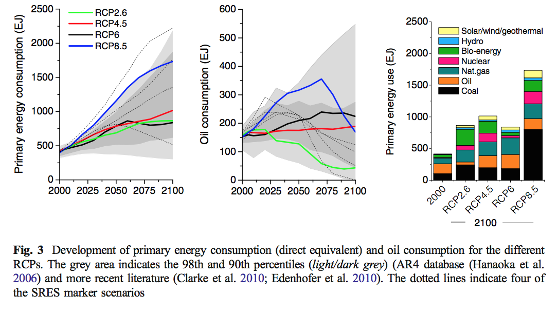
Figure 2 – Click to expand
Annual emissions:
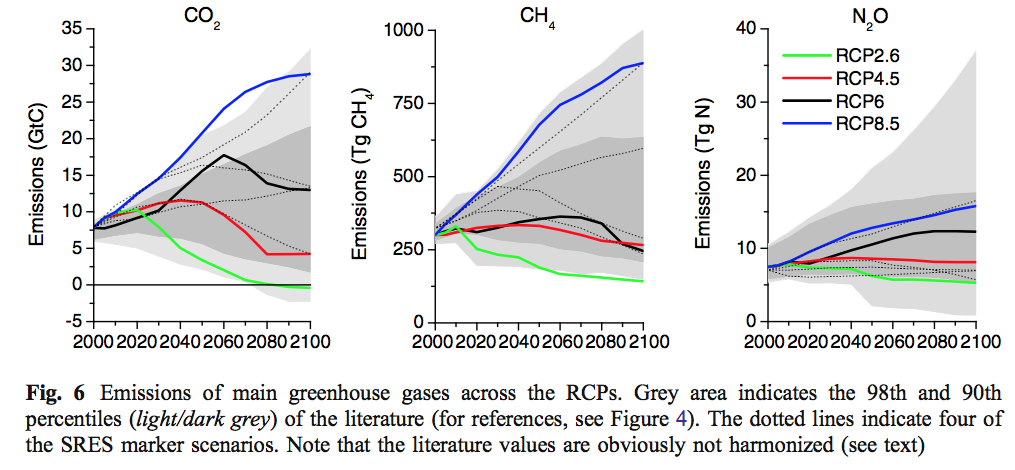
Figure 3 – Click to expand
Resulting concentrations in the atmosphere for CO2, CH4 (methane) and N2O (nitrous oxide):
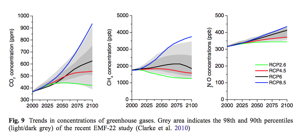
Figure 4 – Click to expand
Radiative forcing (for explanation of this term, see for example Wonderland, Radiative Forcing and the Rate of Inflation):
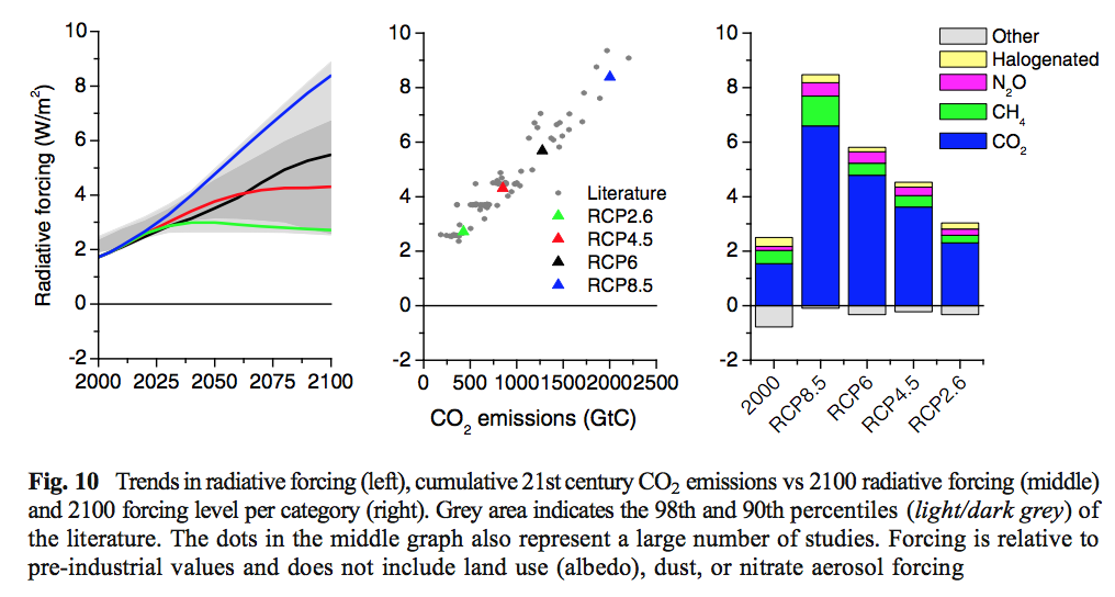
Figure 5 – Click to expand
We can see from this figure (fig 5, their fig 10) that the RCP numbers refer to the expected radiative forcing in 2100 – so RCP8.5, often known as the “business as usual” scenario has a radiative forcing, compared to pre-industrial values, of 8.5 W/m². And RCP6 has a radiative forcing in 2100, of 6 W/m².
We can also see from the figure on the right that increases in CO2 are the cause of almost all of most of the increase from current values. For example, only RCP8.5 has a higher methane (CH4) forcing than today.
Business as usual – RCP 8.5 or RCP 6?
I’ve seen RCP8.5 described as “business as usual” but it seems quite an unlikely scenario. Perhaps we need to dive into this scenario more in another article. In the meantime, part of the description from Riahi et al (2011):
The scenario’s storyline describes a heterogeneous world with continuously increasing global population, resulting in a global population of 12 billion by 2100. Per capita income growth is slow and both internationally as well as regionally there is only little convergence between high and low income countries. Global GDP reaches around 250 trillion US2005$ in 2100.
The slow economic development also implies little progress in terms of efficiency. Combined with the high population growth, this leads to high energy demands. Still, international trade in energy and technology is limited and overall rates of technological progress is modest. The inherent emphasis on greater self-sufficiency of individual countries and regions assumed in the scenario implies a reliance on domestically available resources. Resource availability is not necessarily a constraint but easily accessible conventional oil and gas become relatively scarce in comparison to more difficult to harvest unconventional fuels like tar sands or oil shale.
Given the overall slow rate of technological improvements in low-carbon technologies, the future energy system moves toward coal-intensive technology choices with high GHG emissions. Environmental concerns in the A2 world are locally strong, especially in high and medium income regions. Food security is also a major concern, especially in low-income regions and agricultural productivity increases to feed a steadily increasing population.
Compared to the broader integrated assessment literature, the RCP8.5 represents thus a scenario with high global population and intermediate development in terms of total GDP (Fig. 4).
Per capita income, however, stays at comparatively low levels of about 20,000 US $2005 in the long term (2100), which is considerably below the median of the scenario literature. Another important characteristic of the RCP8.5 scenario is its relatively slow improvement in primary energy intensity of 0.5% per year over the course of the century. This trend reflects the storyline assumption of slow technological change. Energy intensity improvement rates are thus well below historical average (about 1% per year between 1940 and 2000). Compared to the scenario literature RCP8.5 depicts thus a relatively conservative business as usual case with low income, high population and high energy demand due to only modest improvements in energy intensity.
When I heard the term “business as usual” I’m sure I wasn’t alone in understanding it like this: the world carries on without adopting serious CO2 limiting policies. That is, no international agreements on CO2 reductions, no carbon pricing, etc. And the world continues on its current trajectory of growth and development. When you look at the last 40 years, it has been quite amazing. Why would growth slow, population not follow the pathway it has followed in all countries that have seen rising prosperity, and why would technological innovation and adoption slow? It would be interesting to see a “business as usual” scenario for emissions, CO2 concentrations and radiative forcing that had a better fit to the name.
RCP 6 seems to be a closer fit than RCP 8.5 to the name “business as usual”.
RCP6 is a climate-policy intervention scenario. That is, without explicit policies designed to reduce emissions, radiative forcing would exceed 6.0 W/m² in the year 2100.
However, the degree of GHG emissions mitigation required over the period 2010 to 2060 is small, particularly compared to RCP4.5 and RCP2.6, but also compared to emissions mitigation requirement subsequent to 2060 in RCP6 (Van Vuuren et al., 2011). The IPCC Fourth Assessment Report classified stabilization scenarios into six categories as shown in Table 1. RCP6 scenario falls into the border between the fifth category and the sixth category.
Its global mean long-term, steady-state equilibrium temperature could be expected to rise 4.9° centigrade, assuming a climate sensitivity of 3.0 and its CO2 equivalent concentration could be 855 ppm (Metz et al. 2007).
Some of the background to RCP 8.5 assumptions is in an earlier paper also by the same lead author – Riahi et al 2007, another freely accessible paper (reference below) which is worth a read, for example:
The task ahead of anticipating the possible developments over a time frame as ‘ridiculously’ long as a century is wrought with difficulties. Particularly, readers of this Journal will have sympathy for the difficulties in trying to capture social and technological changes over such a long time frame. One wonders how Arrhenius’ scenario of the world in 1996 would have looked, perhaps filled with just more of the same of his time—geopolitically, socially, and technologically. Would he have considered that 100 years later:
- backward and colonially exploited China would be in the process of surpassing the UK’s economic output, eventually even that of all of Europe or the USA?
- the existence of a highly productive economy within a social welfare state in his home country Sweden would elevate the rural and urban poor to unimaginable levels of personal affluence, consumption, and free time?
- the complete obsolescence of the dominant technology cluster of the day-coal-fired steam engines?
How he would have factored in the possibility of the emergence of new technologies, especially in view of Lord Kelvin’s sobering ‘conclusion’ of 1895 that “heavier-than-air flying machines are impossible”?
Note on Comments
The Etiquette and About this Blog both explain the commenting policy in this blog. I noted briefly in the Introduction that of course questions about 100 years from now mean some small relaxation of the policy. But, in a large number of previous articles, we have discussed the “greenhouse” effect (just about to death) and so people who question it are welcome to find a relevant article and comment there – for example, The “Greenhouse” Effect Explained in Simple Terms which has many links to related articles. Questions on climate sensitivity, natural variation, and likelihood of projected future temperatures due to emissions are, of course, all still fair game in this series.
But I’ll just delete comments that question the existence of the greenhouse effect. Draconian, no doubt.
References
Emissions Scenarios, IPCC (2000) – free report
A special issue on the RCPs, Detlef P van Vuuren et al, Climatic Change (2011) – free paper
The representative concentration pathways: an overview, Detlef P van Vuuren et al, Climatic Change (2011) – free paper
RCP4.5: a pathway for stabilization of radiative forcing by 2100, Allison M. Thomson et al, Climatic Change (2011) – free paper
An emission pathway for stabilization at 6 Wm−2 radiative forcing, Toshihiko Masui et al, Climatic Change (2011) – free paper
RCP 8.5—A scenario of comparatively high greenhouse gas emissions, Keywan Riahi et al, Climatic Change (2011) – free paper
Scenarios of long-term socio-economic and environmental development under climate stabilization, Keywan Riahi et al, Technological Forecasting & Social Change (2007) – free paper
Thermal equilibrium of the atmosphere with a given distribution of relative humidity, S Manabe, RT Wetherald, Journal of the Atmospheric Sciences (1967) – free paper
The Great Escape, Health, Wealth and the Origins of Inequality, Angus Deaton, Princeton University Press (2013) – book
Notes
Note 1: Even if we knew future anthropogenic emissions accurately it wouldn’t give us the whole picture. The climate has sources and sinks for CO2 and methane and there is some uncertainty about them, especially how well they will operate in the future. That is, anthropogenic emissions are modified by the feedback of sources and sinks for these emissions.


The BAU terminology goes back to the TAR scenarios. 7.3.2.3 of WG3 says:
“The literature reports several different baseline scenario concepts, including (Sanstad and Howart, 1994; Halsnæs et al., 1998; Sathaye and Ravindranath, 1998):
– efficient baseline case, which assumes that all resources are employed efficiently; and
– “business-as-usual” baseline case , which assumes that future development trends follow those of the past and no changes in policies will take place.”
(BAU is higher than efficient)
So RCP 8.5 was representative of scenarios that had their genesis in these BAU scenarios, and within those was, as per your quote, “relatively conservative”.
I note that I can’t see a reference to the BAU phrase as a description of RCP 8.5 in AR5 WG1.
Looking some more into Riahi et al 2007:
The scenarios shown there relate to the SRES scenarios.
B1 seems to be the “more realistic” one based on the last 50 year trends in rising incomes, large reductions in extreme poverty and consequent reductions in fertility rates.
Population in 2100 is around 7bn:
Click to enlarge
On GDP I have no idea about the various rationals, but I’ve highlighted their B1 scenario which works out to be over US$40,000 per capita globally – compare with today of around $10,000 per capita, and this 2100 estimate is typical rich country GDP per capita of today:
Click to enlarge
Note, I intentionally avoid saying something above like “this means world GDP per capital in 2100 will be $43,689 per person which is 19.5% less than Denmark at $53,698.20 per person” (additional note for pedants, didn’t look up the Denmark figure or calculate the actual values or percentages)
The B1 scenario is matched up with aggressive CO2 reducing tactics embraced by the world, and so is comparable with RCP 4.5.
What would be interesting is to see the B1 scenario with “business as usual” CO2 emissions.
A much lower world population produces lower emissions. A high GDP per capita makes any bad outcomes much more manageable.
Earlier in that paper, p893 of the journal:
Seems like the most useful scenario to explore.
Finally found the SRES – RCP comparison I had been looking for. Better than my hand drawings..
From AR5, chapter 1 (introduction)
Click to expand
Introduction. In: Climate Change 2013: The Physical Science Basis. Contribution of Working Group I to the Fifth Assessment Report of the Intergovernmental Panel on Climate Change, Cubasch et al (2013)
First, all of these scenarios are effectively science fiction. RCP 8.5 is really bad science fiction, sort of like the movie Elysium or the new SyFy channel show Incorporated. The economics and demographics don’t make sense. The world is moving away from coal, not back to it. Even China isn’t going to keep building new coal fired power plants for more than a few decades.
DeWitt,
RCP 8.5 doesn’t make any sense in the light of the last 50 years. It’s as if the world suddenly took a completely different turn and virtually stopped economic development for no reason.
On the plus side, I did watch the first few episodes of Incorporated (on the basis of a recommendation) and I now understand why Hollywood and celebrities are so strongly in favor of urgent action on climate change.
RCP 8.5 in science fiction terms would be what’s called steampunk. In steampunk, technology never made it past the coal fired steam engine. Computers would be based on Babbage’s Difference Engine powered by steam.
https://en.wikipedia.org/wiki/Steampunk
The production design of Emerald City is steampunk based.
Although I’m skeptical about RCP 8.5, it is worth remembering that it is economical to convert coal to petroleum whenever the price of crude oil is above $100/barrel. (The Germans did it during WWII and the South Africans did so during apartheid.) Demand for petroleum is likely to exceed supply for petroleum long before coal runs out. If transportation is still as dependent on petroleum in the second half of the 21st century as it is today, I worry that a lot of fuel could be coming from coal. (Unfortunately, I don’t have any references.)
With regard to the reality of RCP 8.5, current forcings are tracking more closely to RCP 8.5 than to any of the other three scenarios:

In addition, I will note that both Trump in the US, and Turnbull in Australia are currently spruiking a return to coal. It remains a real possibility, although hopefully unlikely.
Tom Curtis,
You’re graph relies on an estimate for 2014. In fact, emissions rose only slightly that year and have been steady, not increasing, since. So it seems more like RCP 6.0 or RCP 4.5.
Tom Curtis,
I don’t think your chart reflects reality. It doesn’t look much like this total emission graph:
Mike M,
All global CO2 emissions data are estimates, including the ones you’re using to dispute the 2014 estimate on Tom Curtis’ chart. There are no actual measurements determining a total amount of CO2 from fossil fuel burning flowing into the atmosphere. It’s all based on economic documentation of processes which would emit CO2.
If we treat the preliminary 2014-2016 estimates as actual then 2016 falls about halfway between RCP8.5 and RCP4.5, but comfortably above RCP6.0. Actually RCP6.0 shows slow near-term growth and only gets up to the current level of emissions in 2030. That’s one reason I don’t think these short term comparisons are necessarily informative for the picture out to 2100.
DeWitt Payne,
The curves look basically the same to me, though obviously yours goes back to 1960 and adds on preliminary estimates for 2015 and 2016.
paulski,
You wrote: “All global CO2 emissions data are estimates … ”
You are playing word games. The axis of the graph is not labelled “estimates”. One point in the graph is labelled “estimate”. That is obviously a different sort of estimate than the others.
I agree that the short term numbers have little relevance for extrapolating to 2100.
I commented with graphics in the newer demographics posting, but relevant points include:
Fertility is lower and falling faster than the UN median variant.
Human population will likely peak lower and sooner than UN median.
Emissions appear to have peaked in 2014.
That stands to reason as some 72% of CO2 emissions are from countries with lower than 2.1 fertility rates.
Aging and falling population will have a dramatic effect on demand just about everything, including fossil fuels ( and energy in general ).
This will be a benefit ( if you think we benefit from slowing CO2 ) but also a curse from slowing economic growth and societal disruption.
The RCP 8.5 CO2 atmospheric CO2 concentration for 2016 is 404.3 ppmv. For RCP 4.5 it’s 402.2. Muana Loa current estimate for 2106 is 404.2. However, the recent El Nino cause a spike in the rate of increase. (See the graph here) I don’t think it’s possible to say with any certainty that CO2 is following RCP 8.5 more closely than RCP 4.5. The current divergence between the different pathways is just too small.
The atmospheric concentrations for 2016 for RCP 6 and 2.6 are 401.4 ppmv and 403.0 ppmv.
Mike M,
Referring to preferred estimates as “facts” and less liked estimates as “estimates” would be an example of playing with words. Referring to all estimates as “estimates” cannot be playing with words.
We can go back to the source of the graph to get some idea of what was meant. It was a commentary first published in late September 2014, which means it was showing a 2014 estimate with data only available perhaps up to halfway through the year. That’s why 2014 was highlighted. It’s not clear they’re using the word ‘estimate’ as an informal labeling distinction from other years in the record, but it’s possible. I would suggest “forecast” would have been a more appropriate word if it is the case.
In any case, estimates of 2016 emissions at this point stem from nearly equally incomplete data, while 2014 and 2015 estimates are generally considered preliminary because data is still coming in and they could change by a relatively substantial amount – about 1% to 1.5%. So if you want to draw a reasonable distinction between solid estimates and incomplete estimates, pretty much everything from 2014 on falls in the latter category at this time. That’s why 2014-2016 are marked with dots on DeWitt’s chart.
Paulski0,
I’ve never looked into how emissions are estimated. If growth from China had slowed a lot in the last few years but they reported “stellar growth, doing great” would the China emissions be inaccurate? I hear that China data is not reliable vs what you might get from Europe or the US with government statistical offices in US/Europe having some measure of independence from politicians.
The graph above on estimated concentrations (my figure 4, their fig 9) is hard to make out in detail, but using the “squinting method” it looks like start of 2017, 404ppm is a little below RCP8.5. Maybe that’s a hopeful squint.
There’s probably source data accessible somewhere for the lines on that graph..
You’re getting way too hung up on the specific details of the RCP8.5 scenario described in that paper. That was just created to fulfil the representative forcing criteria. Look at A1f1 from SRES. 2100 Population about 7 billion, rapid economic growth. 2100 co2 concentration of 1000ppm.
Your understanding of population projections may be a bit behind the times. They’ve been continually revised upwards over the past decade. The current most cited are from the IIASA and the UN, with 2100 medians of 9 billion and 11.2 billion respectively. 95% bound allows up to 12.5 billion in both.
First, all of these scenarios are effectively science fiction. RCP 8.5 is really bad science fiction Agree DWP.
How can intelligent people make such junk? All the scenarios are deeply misleading. The availability and cost of carbon fuel will change. The 0,5% increase pph CO2 will change. There is some peak oil, gas, and coal.
From a paper om peak carbon: Abstract:
“Climate projections are based on emission scenarios. The emission scenarios used by the IPCC and by mainstream climate scientists are largely derived from the predicted demand for fossil fuels, and in our view take insufficient consideration of the constrained emissions that are likely due to the depletion of these fuels. This paper, by contrast, takes a supply-side view of CO2 emission, and generates two supply-driven emission scenarios based on a comprehensive investigation of likely long-term pathways of fossil fuel production drawn from peer-reviewed literature published since 2000. The potential rapid increases in the supply of the non-conventional fossil fuels are also investigated. Climate projections calculated in this paper indicate that the future atmospheric CO2 concentration will not exceed 610 ppm in this century; and that the increase in global surface temperature will be lower than 2.6 °C compared to pre-industrial level even if there is a significant increase in the production of non-conventional fossil fuels. Our results indicate therefore that the IPCC’s climate projections overestimate the upper-bound of climate change”
The implications of fossil fuel supply constraints on climate change projections: A supply-side analysis
Jianliang Wanga, , , Lianyong Fenga, , Xu Tanga, , Yongmei Bentleyb, , Mikael Höökc,
Nobody: Supply-side analysis has been predicting a peak in oil production for the last 40 years or so. Projections based on demand have been superior in the past. Recent low prices have arisen because of lower than expected demand since the financial crisis. So it is clear that today, supply is being driven by demand and that a shortage would be due to underestimation of demand (or OPEC production cuts), not inadequate supply. I don’t know for how many decades this will continue to be true, but it doesn’t make sense to underestimate human ingenuity when there is money to be made meeting demand.
Furthermore, if the authors of your paper are correct, the price of petroleum will rise rapidly. Instead of spending money to cut emissions to avoid warming, we will be spending as much(?) for our limited supply of expensive petroleum products. Not having enough fossil fuel to reach more than 600 ppm of CO2 in the atmosphere will have drawbacks.
Frank,
I’m not a student of peak oil but I think it was a biography of Calvin Coolidge that I read (president in 1920s) where one challenge ahead was peak oil expected in the 1930s. Coolidge: An American Enigma, Robert Sobel.
SOD: To clarify,
a) those who project future oil consumption based on existing reserves are often projecting peak oil in about 20 years.*
b) those – presumably including the IPCC – who project consumption based on demand rising with economic growth are predicting we will never reach peak oil.
Given the finite accessible petroleum deposits from the Carboniferous Period, someday Group b) will stop being right and Group a) will be right for the first time.
Given that coal can be converted to petroleum products, peak oil doesn’t imply peak CO2 emissions from transportation and sectors that currently depend on petroleum. Anytime you use coal in place of other fossil fuels, you release more CO2 for the same amount of energy. So we could have peak oil before 2050 and not have the supply limitations reduce emissions.
* Why 20 years? If oil companies have enough reserves to meet demand for the next 10-20 years, they won’t be investing much in exploration. If they don’t, they will be investing heavily. Historically, those investments have paid off in increasing reserves. However, the size of their recoverable reserves also varies with price.
On peak oil and related energy supply issues, I think this paper may have been linked from a blog article recently (it was sitting in one of many open tabs on my browser):
The implications of fossil fuel supply constraints on climate change projections: A supply-side analysis, Jianliang Wang et al, Futures (2016).
Of course I can’t help but enjoy the accuracy. The above quote has global temperature change at 2.63’C in 2100. More accuracy follows:
This kind of accuracy is worth paying attention to.
If they had said: “..global production will peak 10-20 years from now at 10-15 Gtoe/yr and the cumulative probability.. is over 90%” I would have shaken my head in frustration at their slipshod accuracy.
I don’t know if this paper is an outlier (in content, rather than fake accuracy).
Worth digging in some more at a later date.
So the supply side model that nobobysknowledge cites would be pretty close to RCP 4.5. Demand side models are in the neighborhood of RCP 6.0, according the paper describing the choice of scenarios (van Vuuren et al, 2011). The latter models might be generally more accurate, but don’t really allow for major innovations (as opposed to incremental development). So my guess is that RCP 4.5 is likely to be closer.
By the way, 610 ppm CO2 would be about 1.6 K warming using a TCR of 1.3 K, or 2.1 K using a ECS of 1.8 K.
SOD: I’m interested in how much projected warming will be due to reductions in sulfate aerosols rather than the increase in GHGs. Aerosol forcing supposedly negates 25-75% of the forcing from the rise in CO2. In your Figure 5 (Figure 10 from your source), the gray negative bars could be negative aerosol forcing. If so, the RCP 8.5 (scenario) – but not the others – has aerosols returning to pre-industrial levels.
Thanks to your graphs, I can now see that the future fate of current aerosol cooling (which is bigger than 1 W/m2 in some AOGCMs) is going to be minor compared with 5 or 6 W/m2 of forcing from increased CO2 in RCP6.0 and 8.5.
Frank,
The key word is ‘supposedly.’ Nobody really knows. We do know that aerosols have been used as fudge factors to make high climate sensitivity models fit the historical record. If the GLORY satellite launch had been successful, we would probably know more today. But it wasn’t and there don’t seem to be any plans to replace it. It’s almost like they don’t really want to know.
DeWItt: Doesn’t supposedly cover the scientifically sensible range. If the aerosol indirect effect were zero, would aerosol forcing negate less than 25% of current CO2 forcing?
On the other extreme, aerosol forcing could be negating all of current GHG forcing and 20th century warming could have all been naturally-forced and/or unforced. You don’t support this possibility, do you?
So, I shouldn’t have said “supposedly 25-75%; I probably should have said “25-75%”.
The problem comes from those high-ECS GCMs that reproduce the historical record of warming by using unrealistically high sensitivity to cooling by aerosols and/or high ocean heat uptake.
Frank,
Aerosols negating a very small fraction of ghg forcing with a climate sensitivity at the low end of the IPCC range and with the rate fluctuations in the twentieth century caused by an unmodeled multidecadal oscillation is, IMO, far more probable than aerosols negating nearly all the ghg forcing until the 1950’s with a climate sensitivity in the high end of the IPCC range.
I find it difficult to believe that aerosols had a multidecadal oscillation with a period of ~65 years.
My SWAG would be: not much.
With regard to population, the most recent “official” source I could find currently (2015) projects a 2100 population between 9.5 and 13.3 billion in 2100. The argument that increased wealth results in a birth rate declining to just below replacement values is premised on the experience within just a few cultures. I know that as I grew up in Africa, my neighbours used increase wealth to have multiple wives and children (3 and 21 respectively on one side when I left, 2 and about 9 on the other). Consequently, while I hope that birth rates will decline with affluence, I am not confident
Tom,
I believe it’s every culture.
Of course, individual families vary. However, taking groups as a whole, increased wealth leads to less children – at least this is my understanding. It will be interesting to find some more data. As I was researching the emissions scenarios I also checked the UN projections and saw the high population projections for 2100. I don’t know what assumptions are built into the UN projection.
SoD,
I’ve read that the tie between economic development and fertility rate is not as tight as often assumed. For instance, in the 18th century fertility rates in England dropped more slowly than for many continental countries that lagged behind England in economic development. I don’t have a handy source for that, but from Wikipedia I see that from 1851 to 1901 the population of England roughly doubled while the population of France increased by 10%. I don’t think that difference in net migration could account for that difference.
p.s. I think that it is generally true that every culture eventually undergoes the demographic transition. But some do it early while others do it late.
Mike,
There are a couple of big differences (at least) between the last 50 years and the mid 19th century.
One is contraceptive options – what were they like in 1850?
The other is infant mortality – the US in 1900 had infant mortality of 15%. The US was one of the richest countries at that point and yet today the countries that are still relatively poor, have much better figures for infant mortality.
A typical rich country figure today is less than 0.5% infant mortality. China is 1%, Vietnam 2%, India 4% and scanning through some world bank numbers I couldn’t see any that were as high as the US in 1900.
When you expect all of your children to survive into adulthood and you are prosperous enough not to need them for basic survival (e.g. working on the farm) – and you have the simple technology to allow it – family size starts dropping.
Certainly by the time a country reaches middle income status (>US10,000 per capacity) it’s birth rate always falls: https://upload.wikimedia.org/wikipedia/commons/thumb/d/da/TFR_vs_PPP_2015.png/640px-TFR_vs_PPP_2015.png
There are some cultural differences, but the drop in birthrate between extreme poverty and middle income is enormous. Economic development is desperately needed in sub-sahara Africa to avoid many problems, not the least of which is a tripling of population this century.
Max Roser has some good interactive data sets:
https://ourworldindata.org/fertility/
Also indicates the UN projection of fertility at 2.3 in 2045-2050 timeframe.
CIA has current global fertility at 2.4 for 2016 and falling at 0.02 per year.
Should that persist, we’ll be at 2.3 in five years, a quarter of a century ahead of the UN mid range projection.
Another aspect in this is replacement rate.
Developed world replacement is estimated to be at 2.1 and developing world replacement being higher ( greater infant mortality ). Developing world should have a lowering “replacement rate” with continued improving health.
But developed world should have a slightly rise in replacement rate because the average age at which mothers bear their first child is increasing.
[…] « Impacts – II – GHG Emissions Projections: SRES and RCP […]
[…] In Impacts – II – GHG Emissions Projections: SRES and RCP we looked at projections of emissions under various scenarios with the resulting CO2 (and other GHG) concentrations and resulting radiative forcing. […]
[…] In Impacts – II – GHG Emissions Projections: SRES and RCP we looked at projections of emissions under various scenarios with the resulting CO2 (and other GHG) concentrations and resulting radiative forcing. […]
Great to have you posting again.
Re future economic growth, if you haven’t seen it worth a read.
Rise and Fall of American Growth, Gordon.
He projects much slower growth in the developed world (or rather explains the slower growth we are already experiencing).
Yes, it could be dramatic.
Growth ( increase in GDP ) = productivity * producers
If the number of producers is declining, even with average productivity, growth could become shrinkage.
This may be a far worse problem than global warming.
How much of the current global slowdown is due to this?
Some believe that the “debt overhang” from the financial crisis is the cause of recent slow growth. Hopefully growth will accelerate, but the financial crisis may simply have been a coincident factor exposing the new normal of population drag.
What does this say about recent populism? About the decline of the developed world and the potential rise of the undeveloped world?
TE,
I think you’re ignoring the massive changes in manufacturing productivity from automation. The trend in US manufacturing is still upward, it just takes far fewer workers to produce the same amount of stuff. If productivity in the US were at 2000 levels, we would be employing about 9 million more people in 2016 than were actually employed.
Click to access MfgReality.pdf
If Apple moves production of its next model iPhone back to the US from China, it won’t bring many new jobs because the assembly will be completely automated.
I hope that’s right. It’s easy to get melodramatic about things.
But it hasn’t shown up in the productivity numbers yet.
Maybe because developed economies are already service oriented.
Maybe because there’s duplication ( bricks&mortar AND online ).
But whatever the cause, I suspect there will still be upheaval.
Robots don’t go shopping and robots don’t pay taxes.
[…] scenario” but refer to a speculative and hard to believe scenario called RCP8.5 – see Impacts – II – GHG Emissions Projections: SRES and RCP. I think RCP 6 is much closer to the world of 2100 if we do little about carbon emissions and the […]