Feeds:
Posts
Comments

Archive for the ‘Atmospheric Physics’ Category

In his excellent book, A First Course in Atmospheric Radiation, Grant Petty introduces a number of spectral measurements of atmospheric radiation which are very illuminating.

In this article I am going to reproduce them, along with a lot of Petty’s comments and explanations – hard to improve on what he has to say. (See the book recommendation).

For people confused about how the atmosphere absorbs and emits radiation these might be helpful. For people spreading confusion about how the atmosphere absorbs and emits these will be hard to explain.

Grant Petty (2006)

From Grant Petty (2006)

Figure 1 – The atmosphere above Nauru and Alaska under cloud-free conditions

A few basics first of all – if the atmosphere didn’t emit radiation then the upward looking spectrometer would measure a flat line at zero, as the (extremely low) emission from space at 3K would not even register on the spectrometer. (Note 1).

So where we see very low radiance measurements this is because the atmosphere is transparent at these wavelengths/wavenumbers. (Note 2).

Nauru is in the tropical western Pacific where atmospheric temperatures are warm and humidity is high. Barrow is in the Arctic, and so temperatures in winter are very cold and the atmosphere contains only small amounts of water vapor.

1. The two dashed curves are the Planck function (note 3) at the warmest atmospheric emission seen by the spectrometer at each location.

2. In the tropical example there are two spectral regions where the measured radiance is very close to the 300K reference curve: >14 μm (<730 cm-1 ) and <8 μm (>1270 cm-1). Therefore, the atmosphere must be quite opaque in these bands because the radiation is being emitted from the warmest – and, therefore, lowest – levels of the atmosphere. The >14 μm region is the region of strong absorption of CO2 and, above 15 μm, of water vapor, and the <8 μm region is the water vapor region.

3. In the arctic example we can also see these two water vapor regions, but it’s clear that these are somewhat weaker, with variable radiance. This is because the water vapor concentration is much lower in the colder arctic.

4. In the tropical example, in the region from 8 – 13 μm, the radiances are well below the 300K reference curve and in some cases even a little below the 245K reference curve – this is because the atmosphere is quite transparent in this region.

5. In the arctic example this is much clearer. The 8 – 13 μm region (with the exception of 9.6 μm) is almost at zero radiance because, with much lower water vapor concentration, the spectrometer is almost measuring the radiance of space.

6. The 9.6 μm region in both examples is due to ozone emission. It’s not as obvious in the tropical example because water vapor emission extends across this band.

7. The 15 μm band in the arctic example has an interesting feature. At the center of the band the radiance is a little lower than at the edges of the band. Why is this? The center of the band is the most opaque so it should be measuring the temperature of the lowest levels of the atmosphere, almost at the surface. And the edges of the band – a little less opaque – should be measuring the temperature a little higher up. The reason is that in the arctic in wintertime it is very common to see a temperature inversion, where the surface is colder than the atmosphere a few hundred meters above.

Now let’s review a very interesting pair of measurements. One from 20km looking down – with the simultaneous surface measurement looking up:

From Grant Petty (2006)

From Grant Petty (2006)

Figure 2 – Upwards and downwards measurements at the polar ice sheet

Petty now asks a few questions – in the manner of all good textbook writers. I attempt to answer these questions and if I embarrass myself by getting them wrong, please speak up. I know someone will..

a) what is the approximate temperature of the surface of the ice sheet and how do you know?

b) what is the approximate temperature of the near-surface air, and how do you know?

c) what is the approximate temperature of the air at the aircraft’s flight altitude of 20km, and how do you know?

d) identify the feature seen between 9 – 10 μm in both spectra

e) in fig 1 (fig 8.1) we saw evidence of a strong inversion in the near-surface atmospheric temperature profile. Can similar evidence be seen here?

If you want to check your understanding – try and answer the above questions before reading on. Anyway, you can’t rely on my answers..

My answers, for review:

a) the surface temperature is approx. 268K. The atmosphere is most transparent at 900 cm-1 & 1150 cm-1, so, looking downward at these wavelengths we should see the surface emission. And ice, like water, emits at very close to a blackbody at these wavenumbers.

b) the near surface temperature is approx. 268K. Looking upwards where the atmosphere is most opaque (15 μm) we should see the temperature of the atmosphere closest to the surface. At 15 μm we see a temperature of 268K.

c) the approx. temperature of the air at 20km is 225K. Looking downward from the aircraft where the atmosphere is most opaque (15 μm) we should see the temperature of the atmosphere closest to the measurement device. At 15 μm we see a temperature of 225K (corrected Jan 28th, 2014 thanks to Mike B). Note that we don’t want to rely on the brightness temperature seen at the strongest water vapor absorption (<8 μm) because the water vapor concentration is low when the atmosphere is very cold.

d) the feature seen between 9 – 10 μm in both spectra is the ozone absorption. In the downward looking spectrum from the aircraft we see a colder brightness temperature than the rest of the 8 – 13 μm band – because the rest of the band is viewing the surface, while the ozone absorption centered at 9.6 μm sees the atmosphere much closer to the aircraft. Looking upwards from the surface, the rest of that band sees (very cold) space, while the ozone band reflects the temperature of the lower stratosphere, around 235K.

e) No.

Lastly, four satellite spectra (upwards radiance) from different locations:

From Grant Petty (2006)

From Grant Petty (2006)

Figure 3 – Four satellite measurements from different locations

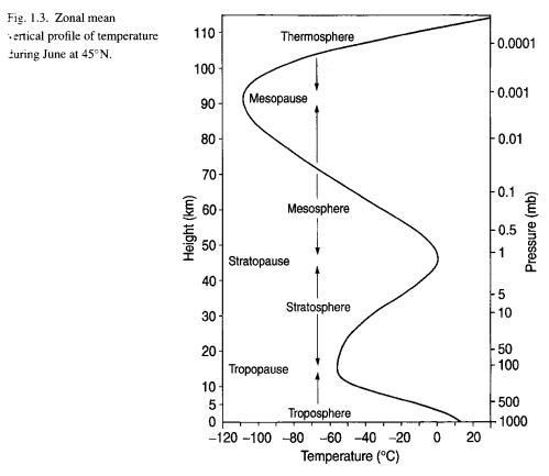
Notice the 15 μm radiance compared with the surrounding band. Remember that the stratosphere warms from the tropopause to the stratopause:

From Grant Bigg (2005)

Figure 4 – Temperature profile of the atmosphere

The reason the brightness temperature (radiance) for the first graph – the Sahara – is at the low temperature of 215K between 14-16 μm is because the satellite is measuring the temperature of the region around the tropopause. But at the very opaque 15 μm the satellite is measuring even closer to itself – higher up in the stratosphere, which is why the brightness temperature is around 230K.

Contrast that with the Antarctic (2nd graph in Fig 3). There we see that the ice sheet is colder than the stratosphere. This is why the 15 μm radiance is higher than the radiance at all the other wavelengths.

If you compare c)  Tropical Western Pacific with d) Southern Iraq you can see the effect of water vapor. In the desert of Southern Iraq where the water vapor is low the radiance is measured from close to the surface – and therefore, is high. In the Western Pacific, where the water vapor concentration is much higher, the radiance is measured from closer to the satellite, i.e., higher up in the atmosphere, where the temperature is lower, and so is the radiance.

Comparing c) and d) for the 15 μm radiance you see that they are almost the same. Water vapor is overwhelmed by CO2 in this region and so water vapor concentration has no effect here.

Conclusion

Even though water vapor and CO2 are present in very low concentrations, they have a very strong radiative effect.

This is not something which is a subject of debate in spectroscopy or in atmospheric physics. The fact that many people find it difficult to understand how a gas present in 360ppm concentrations can have such a strong effect is of no scientific interest. This is because it isn’t a scientific argument.

The changing transparency/emissivity of the atmosphere at various wavelengths provides us with very valuable information about:

a) the concentration of water vapor

b) the temperatures at different heights in the atmosphere

Other articles:

Part One – a bit of a re-introduction to the subject.

Part Two – introducing a simple model, with molecules pH2O and pCO2 to demonstrate some basic effects in the atmosphere. This part – absorption only.

Part Three – the simple model extended to emission and absorption, showing what a difference an emitting atmosphere makes. Also very easy to see that the “IPCC logarithmic graph” is not at odds with the Beer-Lambert law.

Part Four – the effect of changing lapse rates (atmospheric temperature profile) and of overlapping the pH2O and pCO2 bands. Why surface radiation is not a mirror image of top of atmosphere radiation.

Part Five – a bit of a wrap up so far as well as an explanation of how the stratospheric temperature profile can affect “saturation”

Part Six – The Equations – the equations of radiative transfer including the plane parallel assumption and it’s nothing to do with blackbodies

Part Seven – changing the shape of the pCO2 band to see how it affects “saturation” – the wings of the band pick up the slack, in a manner of speaking

Part Eight – interesting actual absorption values of CO2 in the atmosphere from Grant Petty’s book

Part Nine – calculations of CO2 transmittance vs wavelength in the atmosphere using the 300,000 absorption lines from the HITRAN database

Part Ten – spectral measurements of radiation from the surface looking up, and from 20km up looking down, in a variety of locations, along with explanations of the characteristics

Part Eleven – Heating Rates – the heating and cooling effect of different “greenhouse” gases at different heights in the atmosphere

Part Twelve – The Curve of Growth – how absorptance increases as path length (or mass of molecules in the path) increases, and how much effect is from the “far wings” of the individual CO2 lines compared with the weaker CO2 lines

And Also –

Theory and Experiment – Atmospheric Radiation – real values of total flux and spectra compared with the theory.

Notes

Note 1: If it was daytime and the sun was directly overhead (not possible in Barrow, Alaska in March) then the sun’s radiance would add about 1 mW/m2.sr.cm-1 at 1000 cm-1, 1.7 mW/m2.sr.cm-1 at 1400 cm-1 (right hand edge of the graph), and 0.1 mW/m2.sr.cm-1 at 300 cm-1 (left edge of the graph).

Note 2: According to Kirchhoff’s law, if the atmosphere absorbs at any wavelength it also emits at that wavelength – and in equal strength. Absorptivity = Emissivity (but very very important, at the same wavelength, or range of wavelengths). See Planck, Stefan-Boltzmann, Kirchhoff and LTE.

This means that if the atmosphere is transparent at any given wavelength it doesn’t emit at that wavelength. And if it is opaque at any given wavelength it is a strong emitter.

If the absorptivity = 1 at any wavelength (or range of wavelengths) then the emissivity = 1 at that wavelength, meaning it emits like a blackbody at that wavelength.

Note 3: The Planck function is the formula for emission of thermal radiation from a blackbody – a perfect emitter and perfect absorber. There is plenty of unscientific confusion about blackbodies on the web. A blackbody is simply the maximum radiator for any given temperature. Nothing can radiate with a greater intensity at any wavelength than a blackbody and while no real surface is a perfect blackbody many surfaces come close. For example, the ocean has an emissivity of about 0.96. The atmosphere – at some wavelengths – emits very close to a blackbody, while at other wavelengths it is almost transparent and, therefore, the emissivity is close to zero.

Read Full Post »

In this article in the series we will look an interesting paper:

An analysis of the dependence of clear-sky top-of-atmosphere outgoing longwave radiation on atmospheric temperature and water vapor, by Dessler, Yang, Lee, Solbrig, Zhang and Minschwaner, JGR (2008).

This paper can be downloaded for free.

I used some results of this paper in Theory and Experiment – Atmospheric Radiation, but only for comparing calculated top of atmosphere radiative fluxes vs measurement.

I think that the “basic physics” of radiative transfer and atmospheric convection is challenging enough, and the question of feedback even harder.

There are hundreds of papers (thousands really) on this confusing subject and so, for me, drawing conclusions requires a lot of research. Luckily, most people interested in the climate debate already know the answer to the question of feedback from water vapor, so this article won’t be so interesting to them.

In fact, the paper under review doesn’t claim any real answers in the subject of water vapor feedback with climate change:

We are looking at regional variations in lapse rate in a fixed climate, rather than variations in the average lapse rate as the climate changes. This result demonstrates the unsuitability of using variations in different regions in our present climate as a proxy for climate change.

But even with the guarded comments of a published paper, the results are very interesting – and help, at the very least, to illuminate some aspects of how water vapor and atmospheric temperature interact to change the radiative cooling from the planet.

So for people looking for a quick answer, it’s not here. For people wanting to understand the interaction between surface temperature, atmospheric temperature, water vapor and outgoing longwave radiation (OLR) – this might provide a few insights on their journey.

Background

In trying to understand feedback we want to know what happens to the outgoing longwave radiation (OLR) from the climate as surface temperature changes.

Some basic (but hard to calculate) radiative physics – already covered in many places including CO2 – An Insignificant Trace Gas? Part Seven – The Boring Numbers (and the preceding parts of the series) – tells us that, all other things being equal, a doubling of CO2 in the atmosphere from pre-industrial levels will lead to a surface temperature change of about 1°C.

Apart from other variability – how will the climate respond to this increase in surface temperature?

It is only by isolating different causes and effects that we can hope to understand the complexity of the climate. It’s slow but there is more chance of getting the correct answer.

The main miscreant identified as possibly causing a much higher than 1°C increase is water vapor feedback. Water vapor is the dominant “greenhouse” gas, but is variable in space and time as it responds to climate conditions. See, for example, Clouds and Water Vapor – Part Two.

When we think about feedback, one of the most important considerations is how OLR responds to a change in surface temperature.

Let’s consider the change in surface radiation when the temperature increases by 1°C. Most of the earth’s surface has an emissivity very close to 1. At 15°C the increase in surface radiation for this 1°C increase, ΔR = 5.5 W/m². So if the OLR also increased by 5.5 W/m² then the feedback from the climate would be zero. (See comment below for why this is not quite correct).

Why? Because all of the increase in surface radiation has also been emitted from the climate system into space. Picture the scene if instead 10 W/m² was emitted into space after this 1°C increase in surface temperature – this would be negative feedback.

And if the OLR change was 1 W/m² ? This would be positive feedback. Because the increase in radiation from the surface wasn’t matched by radiation from the climate system.

If this doesn’t make sense, ask a question. It’s hard to make progress without grasping this point.

Measurements and “Model”

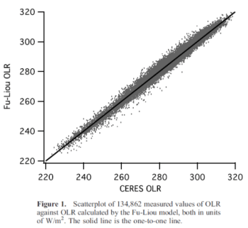
Dessler compares the results of over 100,000 measurements of top of atmosphere (TOA) fluxes from the CERES satellite with two band models which provide computational efficiency (see note 1).

Figure 1 – Comparison of a band model with measured results

This is simply to demonstrate that the model for calculating TOA fluxes is reliable and accurate. The results are used for later calculations. Other graphs in the paper compare the results against surface temperature and latitude to confirm that no bias exists in the results.

Atmospheric temperature and water vapor are measured using AIRS – Atmospheric Infrared Sounder flying on the NASA Aqua satellite. CERES = “Clouds and the Earth Radiant Energy System”, which is also flying on the Aqua satellite.

The measurements taken by AIRS and CERES are “virtually simultaneous”.

These measurements were all taken in March 2005 between 70°N and 70°S over the ocean under clear skies.

The measurements were selected from nighttime measurements. Why? To eliminate any contribution around the 4μm wavelength from solar radiation.

A Basic Equation

Equations aren’t fun for a lot of people and that’s understandable. Stay with me, I will try and explain it in plain English.

What we want to know is how OLR (radiation from the climate to space) changes as surface temperature changes. If we can establish this, we can understand how the climate currently responds to surface temperatures – and what feedbacks are currently in place, at least for the time under consideration:

Figure 2 – The equation

The red term is the main value we want to know – the “rate of change” of OLR with surface temperature

Or, how much does the outgoing longwave radiation change as surface temperature changes?

The orange term = the sum (vertically through the atmosphere) of all the changes in OLR as surface temperature changes, due to the change in atmospheric temperature

The green term = the sum (vertically through the atmosphere) of all the changes in OLR as surface temperature changes, due to the change in water vapor

And before we “dive in”, the basic concepts are, in simple terms:

  • if the atmosphere gets warmer it radiates more to space – and this cools the climate
  • if water vapor increases it reduces the OLR (because it is a “greenhouse” gas) – and this heats the climate (because less radiation to space takes place)
  • if water vapor increases it reduces the “lapse rate” (note 2), making the atmosphere warmer higher up, increasing radiation to space – and this cools the climate

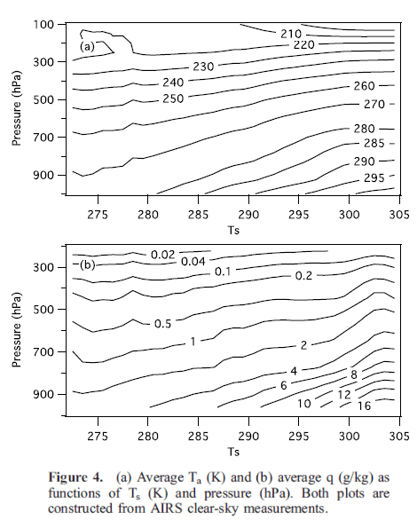
Now let’s take a look at the graphical picture of how atmospheric temperature and humidity vary with surface temperature and height. Think of surface temperature as a proxy for latitude.

Here is how the air temperature vs height, and humidity vs height, vary with surface temperature:

from Dessler (2008)

Figure 3 – Measurements

For those new to humidity measurements in the atmosphere, note the strong dependency on surface temperature and on height in the atmosphere (1000hPa is the surface and 200hPa is around 12km above the surface).

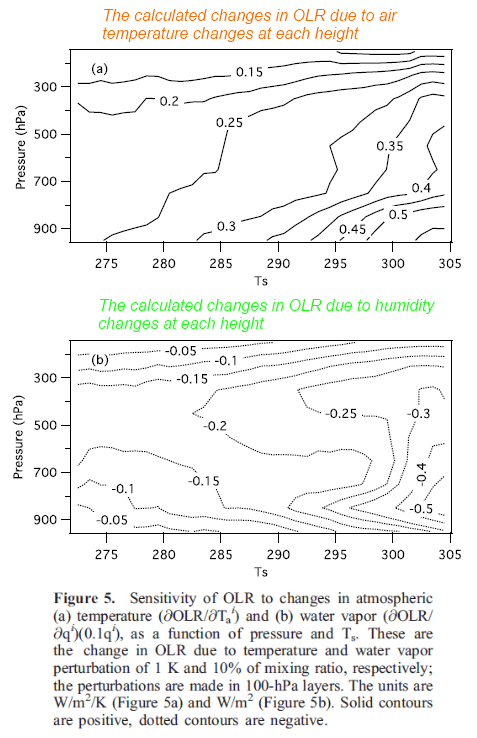
Now we want to plot two of the terms in the equation (figure 2). The colors are matched up with the highlighted terms in the original equation.

From Dessler (2008)

Figure 4 – Calculated – Color text added

These values are calculated by using the model. (We have already seen that this band model accurately calculates the OLR from surface temperature, air temperature and humidity).

As you would expect, when air temperature increases by 1K the OLR increases – because a hotter atmosphere radiates at a higher intensity. This is with all other conditions held the same.

And as you might expect, when the humidity is increased by 10% the OLR decreases – because a more opaque atmosphere has a lower transmittance to surface radiation. This is with all other conditions held the same.

We have been calculating these terms from figure 2:

Now, find how OLR changes due to surface temperature changes we need to also find out these terms:

Or, in English:

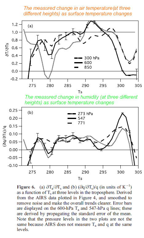
  • the change in air temperature due to surface temperature changes
  • the change in humidity due to surface temperature changes.

From Dessler (2008)

Figure 5 – Measured – Color text added

So, to give an example of what these graphs show, we can see that at around 293-294K, an increase in surface temperature has little or no effect on humidity. Around 300K an increase in surface temperature has a large effect on humidity.

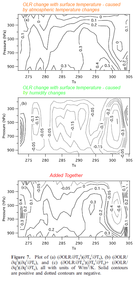
Now we are going to multiply the terms together to find:

  • the change in OLR with surface temperature – due to atmospheric temperature changes
  • the change in OLR with surface temperature – due to humidity changes

Figure 6 – Results – Color text added

The advantage of this method is that when we look at the summary and say, for example:

Oh that’s interesting, the strongest positive feedback effects are around 302 K, what causes that? The strongest negative feedback effects are around 290 – 295 K, what causes that?

– we can review the terms that created the result and see which dominates – and why.

Looking at the total, we can see that between 298 – 303 K the OLR decreases as surface temperature increases (note that the plot is of the change in OLR as Ts increases versus Ts). And below 298 K the OLR increases as surface temperature increases.

This is in agreement with Raval & Ramanathan’s work based on ERBE data shown in Part One where the positive feedback comes from the tropics, and is reduced by the negative feedback from the sub-tropics and mid-latitudes.

The decrease of OLR as surface temperature increases became known as the super-greenhouse effect. Remember that any effect below an increase of 5.5W/m².K (at 15°C) is a positive feedback. (And at 30°C, this threshold value is 6.3W/m².K). An actual decrease of OLR as surface temperature increases is, therefore, a very strong positive feedback effect.

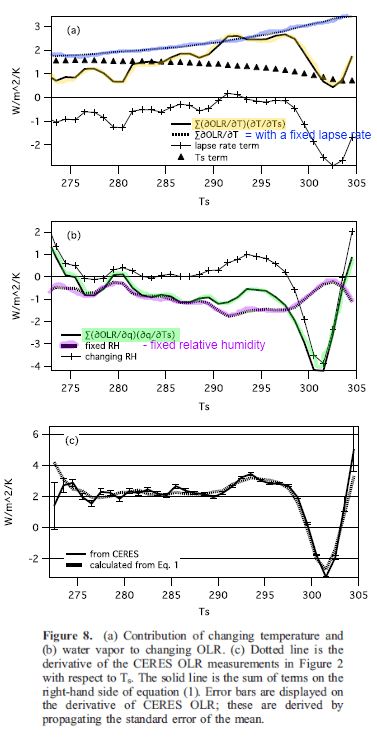
We can see the result plotted against surface temperature and height – now let’s see the total value against surface temperature, and some comparisons of the actuals vs reference scenarios:

Figure 7 – Color text and highlighting added

The first graph shows the change in OLR with surface temperature – due to atmospheric temperature changes. The blue line shows the result if the lapse rate was fixed. Remember that a lower value of changing OLR with Ts is more towards positive feedback.

This is a quantitative estimate of the effect of the changing lapse rate on dOLR/dTs, and it shows that it is negative for almost all values of Ts. In other words, as Ts increases, so does the lapse rate, and the general effect of this is to reduce dOLR/dTs, and therefore OLR, below what they would be if the atmosphere maintained a constant lapse rate.

The second graph shows the change in OLR with surface temperature – due to humidity changes. The purple line shows the result if relative humidity was constant. (And see the results from Sun & Oort, shown in Part Three).

In the subtropics, the ‘‘changing RH’’ line is positive, meaning that RH decreases with increasing Ts. This relative dryness contributes to high values of OLR here, providing a key pathway for the climate system to lose energy back to space. As Ts crosses the convective threshold, ≈298 K, the RH of the atmosphere abruptly increases, leading to a strong increase in q and a reduction in OLR and its gradient.

The third graph compares the results by using the data graphed in Figure 1 with the results derived through this article – and they are the same.

We also plot in this panel the right-hand side of equation (1):

Σi(∂OLR/∂Ti)(∂Ti/∂Ts) + Σi(∂OLR/∂qi)(∂qi/∂Ts) + ∂OLR/∂Ts,

derived from lines plotted in Figures 8a and 8b. As one can clearly see, the agreement is excellent. Note that this is a stringent test as these two lines are derived from completely independent data: one line is derived entirely from CERES data while the other line is derived entirely from AIRS data and a radiative transfer model. The excellent agreement gives us great confidence that, given observations of Ta and q, the clear-sky OLR budget is well understood inthe present atmosphere. We also see no evidence that neglected terms are important, in agreement with previous work..

Conclusion

The paper gives us an excellent insight into how atmospheric temperature and humidity vary as surface temperature varies – over the ocean. And how this maps into changes in OLR as surface temperature changes.

We see that the results are similar to Ramanathan’s work shown in Part One.

These are valuable insights.

If surface temperature increases from any cause, does this mean that positive feedback from water vapor will amplify this? If surface temperature reduces from any cause, does this mean that positive feedback from water vapor will amplify this?

Surely that depends.

But ask yourself this – if the results had shown the opposite effect, would you find them significant?

Articles in this Series

Part One – introducing some ideas from Ramanathan from ERBE 1985 – 1989 results

Part One – Responses – answering some questions about Part One

Part Two – some introductory ideas about water vapor including measurements

Part Three – effects of water vapor at different heights (non-linearity issues), problems of the 3d motion of air in the water vapor problem and some calculations over a few decades

Part Five – Back of the envelope calcs from Pierrehumbert – focusing on a 1995 paper by Pierrehumbert to show some basics about circulation within the tropics and how the drier subsiding regions of the circulation contribute to cooling the tropics

Part Six – Nonlinearity and Dry Atmospheres – demonstrating that different distributions of water vapor yet with the same mean can result in different radiation to space, and how this is important for drier regions like the sub-tropics

Part Seven – Upper Tropospheric Models & Measurement – recent measurements from AIRS showing upper tropospheric water vapor increases with surface temperature

Notes

Note 1: See CO2 – An Insignificant Trace Gas? Part Four for more explanation of “band models”. A “model” doesn’t mean “GCM”. In this case it simply means a more efficient way of calculating the TOA flux than using “line by line” calculations in the radiative transfer equations.

The HITRANS database contains 2.7M spectral lines and so “doing it the long way” takes a lot of time. Therefore, over time, many band models have been created – and critically evaluated – against the hard way.

Note 2: The lapse rate is the decrease in temperature as you go up through the atmosphere. In a dry atmosphere the temperature reduces at around 10K/km. In a very moist atmosphere the temperature reduces at around 4K/km. And, on average, the lapse rate is 6.5K/km. So the more water vapor there is in the atmosphere, the warmer the atmosphere at any given height.

Read Full Post »

In the last article we looked at some results from Grant Petty.

In essence they demonstrate the huge variation in the transmittance of CO2 through the atmosphere with the wavelength of radiation.

I decided it might be interesting to try and reproduce these results using the HITRAN database. This allows a closer examination of which mechanisms cause which results.

Line Shapes and Pressure Broadening

The energy in a photon is given by a very simple equation:

E = hν

where h = Planck’s constant = 6.63 x 10⁻³⁴ J.s, and ν = frequency (ν=c/λ where c=speed of light and λ = wavelength)

So, for example, a 15μm photon has an energy of 1.3 x 10⁻²⁰ J.

A photon can be absorbed by a molecule if the energy of the photon matches the exact energy required to change the state of that molecule.

Now, if a photon was only absorbed at one exact wavelength then atmospheric radiation would be irrelevant.

An easy concept for people who have done a lot of maths or physics, but not so obvious to many others.

Let’s take a different example. If you start your car up and accelerate steadily up to 60 miles per hour over 1 minute, how long do you spend at the speed of 34.5698895549034592345123 miles per hour? Not much. And the more precise I make this speed, the less time you will have spent at it.

If we consider how much energy is transferred in terrestrial radiation from the surface at 14.995698895549034592345123 μm, the answer is “not much”. The same goes for any other vanishingly small interval of wavelengths.

So if each absorption line was exactly one wavelength then the amount of energy absorbed by a finite number of lines would be zero.

However, each absorption line has a finite width. Part of this is due to the uncertainty principle described by quantum mechanics – the small time a higher energy state is occupied produces an uncertainty in the energy of that state.

This is called natural broadening and is a very small effect.

The easiest broadening mechanism to understand is Doppler broadening. Molecules in the atmosphere are zipping around in all directions at speeds of around 500 m/s. Compared with the speed of light this is small, but the difference in the relative speed between a photon and a molecule is slightly changed, leading to a change in the absorption frequency (see note 1 for more details). This is “relatively easy” to understand from first principles and the mathematical treatment is straightforward.

The dominant line broadening mechanism in the lower atmosphere is pressure, or collisional, broadening. This is more challenging from a theoretical point of view but is certainly a measurable value.

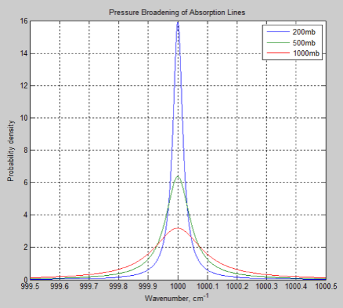
The main effect of pressure broadening is to “spread out” the absorption line. Here is a typical example, where 1000mb is at the earth’s surface, and 200mb is at the “tropopause”, or top of the lower atmosphere:

Figure 1

So the absorption at the center of the line is reduced, while more absorption takes place out to the sides.

The parameter which describes how much broadening has taken place is called the half-width – and is the width of the line when the value has dropped to half the peak value.

Typical values of pressure broadening half width are 0.01 – 0.1 cm-1 at 296 K and pressure of 1000 mb (surface atmospheric pressure).

The function which approximates this effect is the Lorentz line shape:

f(ν-ν0) = αL/π((ν-ν0)²+αL²)       [1]

where ν0 is the frequency of the absorption, ν = frequency and αL = half-width at half of the maximum

And the half-width at any given temperature and pressure is given by this formula:

αL = α0(p/p0).(T0/T)γ [2]
where α0 = lab measured half-width at pressure p0 and temperature T0, and γ is also a lab measured parameter, typically around 0.5 – 0.7.

That’s a lot to take in if you haven’t seen it before. Take a look back at Figure 1 – this is what these formulas describe.

The atmospheric pressure where pressure broadening is comparable to Doppler broadening is about 10 mbar. This is around 30km above the surface, so in the troposphere Doppler broadening is unimportant.

In a later article we might explore the experimental results vs theoretical results of pressure broadening in more detail. Or at least, how much inaccuracies might affect radiative transfer calculations.

HITRAN database

You can read more about the HITRAN database here. The most recent update of the database is described in The HITRAN 2008 molecular spectroscopic database, by L.S. Rothman et al, and the earlier 2004 update: The HITRAN 2004 molecular spectroscopic database, by L.S. Rothman et al.

This database is the result of a huge amount of work by thousands of researchers over a few decades. If you look at the references in the 2008 paper you find almost 400 papers.

In the previous articles in this series I created two fictitious molecules, pCO2 and pH20, and solved the radiative transfer equations for a variety of conditions for these two molecules through the atmosphere.

The aim of this simplification was illumination.

Given that the HITRAN database contains over 300,000 absorption lines for CO2 (and 2.7M lines in total), I thought that replicating some standard results (e.g. see Part Eight) might be a little too much of a challenge. However, the hardest part was actually reading the database, which is in text form – and the problems were just due to my novice status with MATLAB.

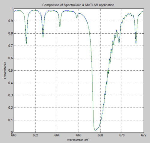
DeWitt Payne kindly offered me some results he obtained from SpectralCalc (via subscription). These were from 660-672 cm-1 through a 1 meter path at standard temperature and pressure, and CO2 concentrations of 380 ppm.

Here is the comparison with my MATLAB program:

Figure 2

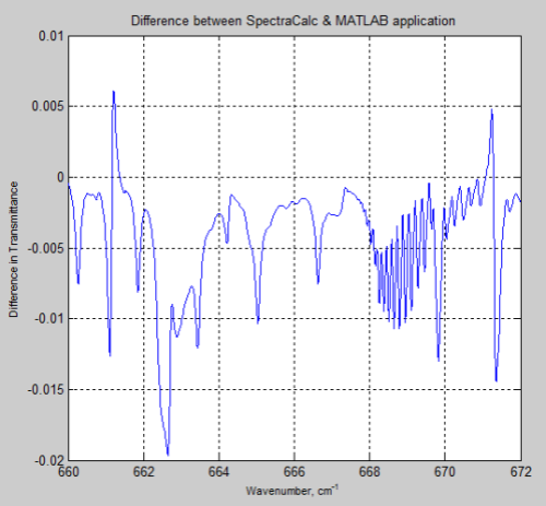
And here is the difference between the two results (the SpectralCalc results minus the MATLAB results):

Figure 3

The MATLAB program, for the results above, only considered the main isotopologue of CO2, which accounts for over 98% of the concentration of CO2 in the atmosphere. However, including the absorption lines for all isotopologues had almost no effect and the small differences remain.

As the differences are small, it seems worth showing some initial results from the program.

Results

First, let’s see the effect of “pressure broadening”.

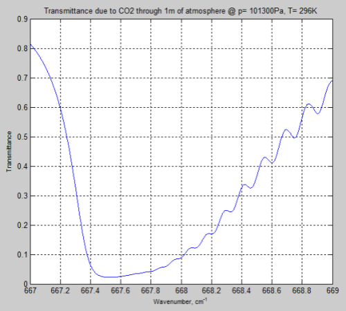
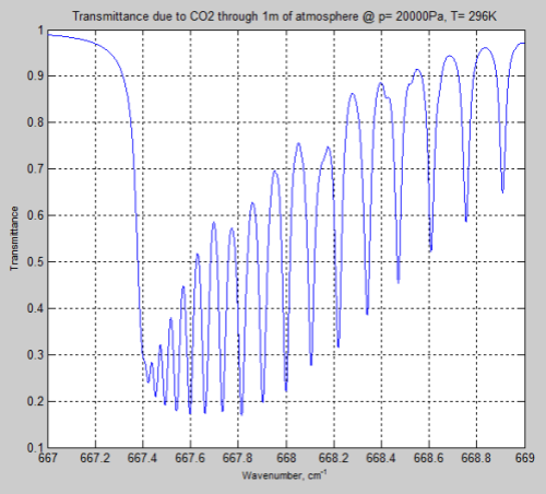
Here is the result through 1m of atmosphere at the earth’s surface, around the peak absorption wavenumber of CO2:

Figure 4

And the result for the same 1m of atmosphere at the tropopause (top of the troposphere) at 200mbar (typically around 12km):

Figure 5

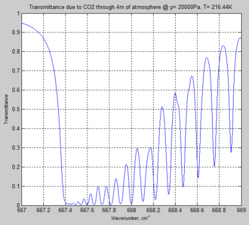
Now at 200 mbar there is less atmosphere so the comparison isn’t truly a fair one. Increasing the path length to get the same number of CO2 molecules we get this result:

Figure 6

Both pressure and temperature have changed so it’s worth seeing the result if we apply the surface temperature to the Figure 5 results:

Figure 7

We can see from the result (and it’s also clear from the equations earlier) that the parameter having the most effect is the pressure – which changes by a factor of 5. The temperature reduction from 296K to 216K has a much smaller impact.

However, the difference between Figure 4 and Figure 6 is very significant – individual lines are “smeared out” at the earth’s surface, but distinct lines higher up in the atmosphere.

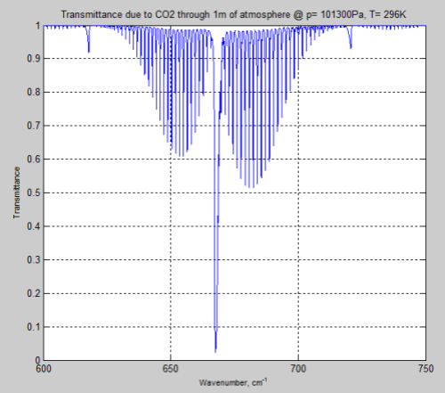
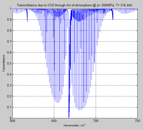
Let’s take a look at a wider range of wavenumbers / wavelengths.

From 600 – 750 cm-1 (13.3 – 16.7 μm) at the surface through 1 meter of atmosphere:

Figure 8

And the same amount of CO2 at the tropopause:

Figure 9

Let’s look at a longer path of 100m through the atmosphere and “zero in” on one part of the bandwidth, 640-650 cm-1:

Figure 10

And let’s compare it with the tropopause, again through a longer path, to keep the CO2 quantity the same:

Figure 11

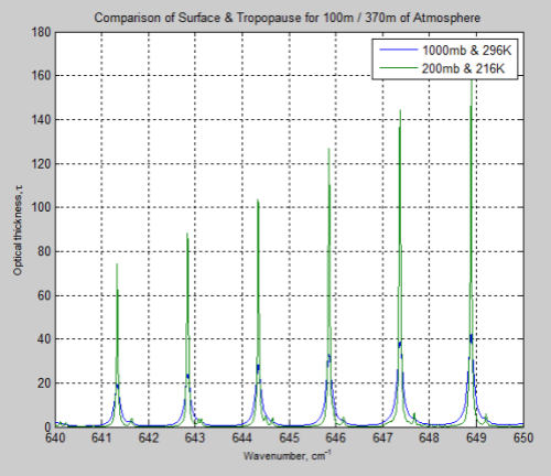
Just for interest I compared the optical thickness of the surface and tropopause for these wavenumbers on the same graph. Optical thickness increases as transmittance decreases. Check out the heading Optical Thickness & Transmittance in Part Six if this isn’t clear.

Figure 12

We can see that the peaks of absorption are indeed lower but the widths of the absorption lines are wider (for the surface results).

Saturation Revisited

As I commented in Part Eight, many people have heard about the high absorption of CO2 at 15 μm and have not understood the huge variation in absorption across the wide bandwidth of CO2. (Also there is the most important subject of re-emission).

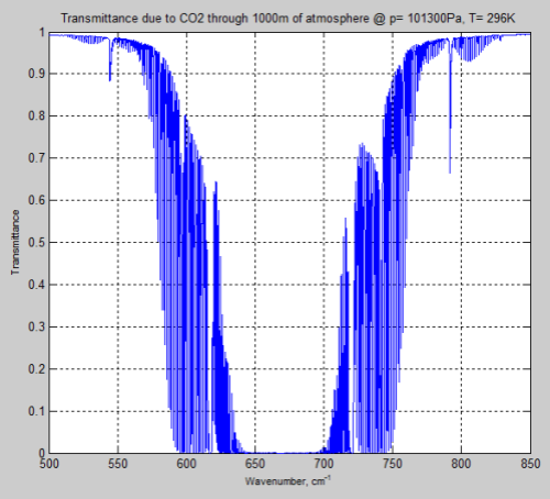
Here is the result of the simple “slab” model, which calculates the transmittance through 1km of atmosphere (a slab model means that the pressure and temperature are constant through the “slab” – a very simple model):

Figure 13

As you can see, around 570 – 600 cm-1 (16.7 – 17.5 μm) and 730 – 770 cm-1 (13.0 – 13.7 μm) the transmittance through the atmosphere is nowhere near “saturated”.

If 1 km of atmosphere has a transmittance of 0.7 (i.e., 70% of radiation is transmitted) at some wavelengths then clearly more CO2 will reduce this transmittance.

The Matlab Code

The results were all created using my code: HITRAN_0_2. However, each run has slightly different parameters, which are adjusted by changing the code rather than anything more elegant. See Note 2 for the code.

The code at this stage has provision for different layers of different temperatures, pressures, and densities – but at this stage the code doesn’t use it – just one “slab”.

The core part of the code is very simple:

  • Take each absorption line in turn and use its measured line strength, half width, and other parameters
  • For the pressure and temperature, calculate the half width for those conditions (equation 2)
  • Now for each line, take each wavenumber in turn (defined via a start, stop and interval) and apply the formula in equation 1 to calculate the optical thickness
  • Add the optical thickness at this wavenumber to the optical thickness already calculated for this wavenumber

The code could be more “speed efficient” – by only calculating equation 1 close to the absorption line. I started out simpler to see what happened and it went so fast that I didn’t improve it.

Multiple Atmospheric Layers

As the pressure and temperature change with height through the atmosphere the single slab model is limited in value.

So I extended the model to multiple layers – v0.3 (see Note 2).

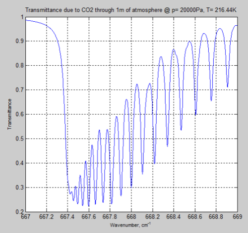
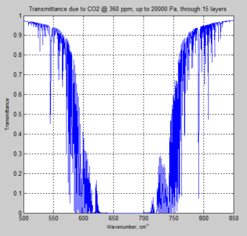
Here is the result of transmittance up to 200mb (20,000 Pa) from CO2 at 360 ppm with a 15 layer model:

Figure 14

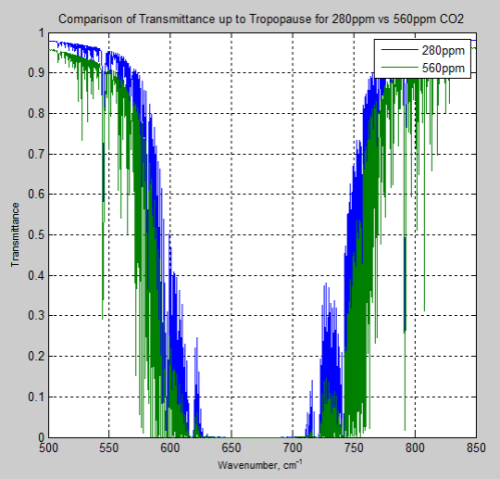
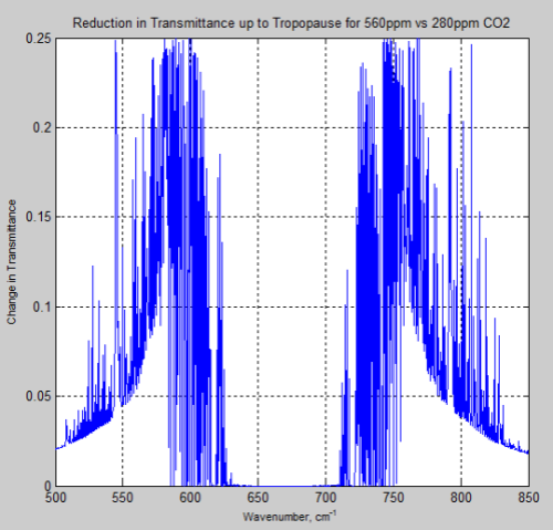
And, of course, the question many people have – what is the difference between the atmosphere at 280 ppm and 560 ppm – or a doubling of CO2 from pre-industrial levels:

Figure 15

And the difference between the two, the “delta”:

Figure 16

Remember – or note, if this is new – the atmosphere absorbs and also re-emits. The question of radiative forcing cannot be answered by only considering transmittance.

However, these graphs of the change should at least indicate to people that the issue of the very high optical thickness = very low transmittance at 667 cm-1 = 15 μm is not the complete story, even only considering transmittance.

Limitations

The model has the limitation at the moment that it doesn’t take into account Doppler broadening. If we extend the model up into the stratosphere Doppler broadening starts to become important. I might get around to including this by introducing the Voigt function which combines pressure broadening and Doppler broadening.

There is also the possibility that my model has a mistake. However, I have compared it to the results from SpectralCalc and it is very close, and to results published in Grant Petty’s book, which look the same.

Other articles:

Part One – a bit of a re-introduction to the subject.

Part Two – introducing a simple model, with molecules pH2O and pCO2 to demonstrate some basic effects in the atmosphere. This part – absorption only.

Part Three – the simple model extended to emission and absorption, showing what a difference an emitting atmosphere makes. Also very easy to see that the “IPCC logarithmic graph” is not at odds with the Beer-Lambert law.

Part Four – the effect of changing lapse rates (atmospheric temperature profile) and of overlapping the pH2O and pCO2 bands. Why surface radiation is not a mirror image of top of atmosphere radiation.

Part Five – a bit of a wrap up so far as well as an explanation of how the stratospheric temperature profile can affect “saturation”

Part Six – The Equations – the equations of radiative transfer including the plane parallel assumption and it’s nothing to do with blackbodies

Part Seven – changing the shape of the pCO2 band to see how it affects “saturation” – the wings of the band pick up the slack, in a manner of speaking

Part Eight – interesting actual absorption values of CO2 in the atmosphere from Grant Petty’s book

Part Nine – calculations of CO2 transmittance vs wavelength in the atmosphere using the 300,000 absorption lines from the HITRAN database

Part Ten – spectral measurements of radiation from the surface looking up, and from 20km up looking down, in a variety of locations, along with explanations of the characteristics

Part Eleven – Heating Rates – the heating and cooling effect of different “greenhouse” gases at different heights in the atmosphere

Part Twelve – The Curve of Growth – how absorptance increases as path length (or mass of molecules in the path) increases, and how much effect is from the “far wings” of the individual CO2 lines compared with the weaker CO2 lines

And Also –

Theory and Experiment – Atmospheric Radiation – real values of total flux and spectra compared with the theory.

References

The HITRAN 2008 molecular spectroscopic database, by L.S. Rothman et al, Journal of Quantitative Spectroscopy & Radiative Transfer (2009)

Notes

Note 1 – The energy absorbed from a photon, E = hv, where h = Planck’s constant, and ν= frequency. The energy of the photon has to match precisely the energy required for the change in state of the molecule.

However, due to the motion of atmospheric molecules, the actual frequency, ν’ = ν(1-ν/c), where c = speed of light, ν = frequency measured by a stationary observer.

In essence, there is now a very small (but measurable) range in frequencies (with respect to a “stationary” planet) that can be absorbed to give the precise energy level required for a transition of this molecule – and so the faster the molecules are moving, the more the absorption line “spreads out”.

Molecular speeds are given by the Maxwell-Boltzmann distribution.

Note 2

HITRAN v0.2

HITRAN v0.3

And the code for v0.2 reproduced here for convenience:

====== HITRAN v0.2 ===================

function [vmin vmax dv cco2 T p d vt tau ] = HITRAN_0_2()

% Absorption through atmosphere of defined temperature & pressure

% uses the HITRANS database

%

% v0.1 – Basic calculations to get out of the starting blocks

% v0.2 – Tidy up and allow a “slab” to be at any pressure and temperature

%       with line width determined by the pressure & temperature

clear

disp([‘—- New Run —- ‘ datestr(now) ‘ —-‘]);

disp(‘  ‘);

% =========== Basic definitions =====================

p0=1.013e5; % std pressure for the HITRANS database in Pa

T0=296; % std temperature for HITRANS database in K

cco2=360e-6; % concentration of CO2

Na=6.02e23; % Avogradro’s number

mair=29e-3; % molar mass of air

% now define the fractional abundance of each isotopologue of CO2

isoprop=[0.98420 0.01106 0.0039471 0.000734 0.00004434 0.00000825 0.0000039573 0.00000147];

ignoreiso=false; % allows easy switching between main isotopologue only or all of them

% =========== Define wavenumber ranges ==============

vmin=640; % min wavenumber to consider (overall)

vmax=650; % max wavenumber to consider (overall)

dv=0.001; % resolution of wavenumber

% because absorption lines below the lower boundary (and above the upper

% boundary) can still affect the wavenumbers under consideration we need to

% extend the boundaries of which absorption lines to consider

rvmin=0.98; % ratio below lower boundary to consider

rvmax=1.02; % ratio above upper boundary to consider

%vt=vmin:dv:vmax; % vt = wavenumbers we will calculate optical depth for

vt=linspace(vmin,vmax,1063);

vtmax=length(vt);

tau=zeros(1,vtmax); % set optical depth to zero as a starting point

% =========== Read in CO2 data and select vmin-vmax data ========

% selected paramaters for complete HITRAN CO2 database already stored in file: co2.mat

load(‘co2’);

if ignoreiso==true

% select only main isotopologue between the wavenumber boundaries

iv=find(iso==1 & v>vmin*rvmin & v<vmax*rvmax); % select upper and lower bounds

else

% select all isotopologues and between the wavenumber boundaries

iv=find(v>vmin*rvmin & v<vmax*rvmax); % select upper and lower bounds

end

% select subset of CO2 spectral data for evaluate

iso=iso(iv); v=v(iv); S=S(iv); gama=gama(iv); nair=nair(iv);

ivmax=length(v);

% ============= Define standard atmosphere against height ================

% reuse code from rte_0_5_0 to define std atmosphere and number of levels

% SI units used unless otherwise stated

% first a “high resolution” atmosphere

% zr = height, pr = pressure, Tr = temperature, rhor = density

Ts=296; % define surface temperature at same value as HITRAN measurements

ps=1.013e5; % define surface pressure

Ttropo=215; % define tropopause temperature

% nmv=2.079e25; % nmv x rho = total number of molecules per m^3, not yet

% used

maxzr=50e3; % height of atmosphere

numzr=5001; % number of points used to define real atmosphere

zr=linspace(0,maxzr,numzr); % height vector from sea level to maxzr

[pr Tr rhor ztropo] = define_atmos_0_3(zr,Ts,ps,Ttropo); % function to determine (or lookup) p, T & rho

% Create “coarser resolution” atmosphere – this reduces computation

% requirements for absorption & emission of radiation

% z, p,Tinit,rho; subset of values used for RTE calcs

numz=10; % number of boundaries to consider (number of layers = numz-1)

minp=2e4; % top of atmosphere to consider in pressure (Pa)

% want to divide the atmosphere into approximately equal pressure changes

dp=(pr(1)-minp)/(numz); % finds the pressure change for each height change

zi=zeros(1,numz); % zi = lookup vector to “select” heights, pressures etc

for i=1:numz % locate each value

zi(i)=find(pr<=(pr(1)-i*dp), 1); % gets the location in the vector where

% pressure is that value

end

% now create the vectors of coarser resolution atmosphere

% z(1) = surface; z(numz) = TOA

% T, p, rho all need to be in the midpoint between the boundaries

% T(1) is the temperature between z(1) and z(2), etc.

z=zr(zi);   % height

pb=pr(zi);   % pressure at boundaries

Tb=Tr(zi);   % starting temperature at boundaries

rhob=rhor(zi);  % density at boundaries

% now calculate density, pressure and temperature within each layer

for i=1:numz-1

dz(i)=z(i+1)-z(i); % precalculate thickness of each layer

Tinit(i)=(Tb(i+1)+Tb(i))/2; % temperature in midpoint of boundary

p(i)=(pb(i+1)+pb(i))/2; % pressure in midpoint of boundary

rho(i)=(rhob(i+1)+rhob(i))/2; % density in midpoint of boundary

end

% ===============

% but in the first version we ignore this and just calculate at std temp

% and pressure (later iterate through each layer, i

% work in cm for volumes and distances (absorption coefficients are in cm)

p=p0;

rhop=rhor(find(pr<=p,1)); % lookup density at pressure = p

T=Tr(find(pr<=p,1)); % lookup temperature at pressure = p

na=(Na*rhop/mair)/1e6; % number of air molecules per cm^3

Nco2=na*cco2; % number of CO2 molecules per cm^3

d=100*100; % path length in cm *** just a starting point

% ======== Iterate through each absorption line ======

% for one slab of depth, d

for j=1:ivmax  % each absorption line

% v(j)=line center, S(j)=line strength, gama(j)=half width

% first do a code inefficient method – calculate the profile for each

% across the entire wavenumber range

if ignoreiso==true   % if we only want to consider the main isotopologue

prop=Nco2;

else

prop=isoprop(iso(j))*Nco2;

end

ga=gama(j).*(p/p0).*(T0/T).^nair(j);

% ======== Iterate through each wavenumber  ====

for k=1:vtmax  % each wavenumber

%  vt(k) is the wavenumber under consideration

dtau=prop*d*S(j)*ga/pi/((vt(k)-v(j))^2+ga^2);

tau(k)=tau(k)+dtau;

end

end

plot(vt,exp(-tau))

title([‘Transmittance due to CO2 through ‘ num2str(round(d/100))…

‘m of atmosphere @ p= ‘ num2str(p) ‘Pa, T= ‘ num2str(T) ‘K’])

ylabel(‘Transmittance’,’FontSize’, 8)

xlabel(‘Wavenumber, cm^-^1′,’FontSize’, 8)

grid on

disp([‘Range = ‘ num2str(vmin) ‘ – ‘ num2str(vmax) ‘ cm^-1, dv = ‘ num2str(dv) ‘, lines = ‘ num2str(ivmax)]);

disp([‘Number of CO2 molecules per cm^3 = ‘ num2str(Nco2) ‘, path length = ‘ num2str(d/100) ‘ m’]);

disp([‘p= ‘ num2str(p) ‘ Pa, T= ‘ num2str(T) ‘ K’]);

disp([‘—- Complete End —- ‘ datestr(now) ‘ —-‘]);

======== end of HITRAN v0.2 =====================

Read Full Post »

I thought some data provided in Grant Petty’s excellent book would be valuable as it helps explain some important points about the role of CO2 in the atmosphere.

Just recently I was kindly given access to the HITRAN database by Dr. Laurence S. Rothman but I’ve spent a bit too much time in the last few days trying to get MATLAB to read it (still a novice at MATLAB). I do plan to provide a followup article with some calculations of my own on the HITRAN data. Who knows how long that will take.

HITRAN is an acronym for high-resolution transmission molecular absorption database. It is a treasure trove of spectroscopic data.

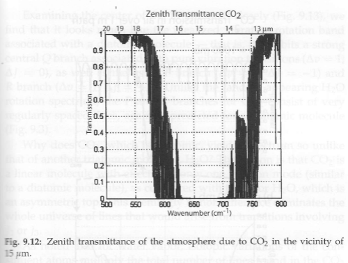
First, here’s a couple of extracts from A First Course in Atmospheric Radiation by Grant Petty. (I briefly reviewed this book in Find Stuff Out and Book Reviews):

From "A First Course in Atmospheric Radiation", Grant Petty (2006)

From "A First Course in Atmospheric Radiation", Grant Petty (2006)

What is “zenith transmittance”?

It is the proportion of radiation that is transmitted (not absorbed or scattered) through the atmosphere from the surface to the top of atmosphere. It doesn’t include any re-radiation by the atmosphere – an important element of atmospheric radiation (see, for example, Part Three).

What is “zenith transmittance of CO2”?

The above effect when only CO2 is taken into account.

This graph is therefore calculated not measured. The only way to measure it would be to take out all the water vapor while the satellite was taking the measurement, which is tricky. It would also be important to stop the atmosphere re-radiating which is even more challenging.

Of course, the calculations are based on the measured parameters of CO2.

Now, the value of this graph is in demonstrating that for much of the CO2 absorption band (e.g. around 600 cm-1 and 750 cm-1) the transmission through the entire atmosphere is not zero and not 1. Therefore, more CO2 will have an effect on the transmittance of the atmosphere.

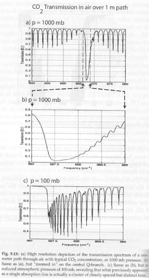
Here’s the value through a 1m path around the better known peak absorption of CO2 at wavenumbers around 667cm-1 = wavelengths around 15μm:

From Grant Petty (2006)

Fascinating stuff. As you can see 95% of radiation at 15μm is absorbed in just 1 meter of atmosphere at the surface of the earth (1000 mb).

Amazing, considering that CO2 is only 370ppm or thereabouts.

You can see the effect of what is called “pressure broadening” of the individual lines with the 1000mb (surface pressure) vs the 100mb (about 16km altitude) value.

This is something we will return to in a later article.

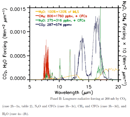
Many people write about the strong absorption of CO2 at 667 cm-1 / 15μm without commenting on the absorption at 600 cm-1 or 750 cm-1.

The less strong absorption around the “wings” of the band is the reason for this graph below of the wavelength dependent impact of a doubling of CO2 (from pre-industrial levels) on the “radiative forcing”:

Longwave radiative forcing from increases in various "greenhouse" gases

Longwave radiative forcing from increases in various "greenhouse" gases

From Radiative forcing by well-mixed greenhouse gases: Estimates from climate models in the IPCC AR4, W.D. Collins et al, Journal of Geophysical Research (2006). Note that the vertical axis units are incorrect.

Early comments on CO2 in the HITRAN database

There are almost 315,000 individual absorption lines for CO2 recorded in the database. The database has 2.7M absorption lines in total for 39 molecules.

Between 665 – 669 cm-1 there are over 2,000 lines.

Between 647 – 687 cm-1 there are over 16,000 lines.

Between 500 – 800 cm-1 (12.5 μm – 20μm) there are almost 63,000 lines.

Over 248,000 lines for CO2 are above 800 cm-1 , i.e., between 0-12.5 μm.

The main reference paper for HITRAN 2008 (see below) says:

The present atmospheric version of CDSD (Carbon Dioxide Spectroscopic Databank) consists of 419,610 lines .. covering a wavenumber range of 5–12784 cm-1.

– so I’m not sure whether not all of them made it into the HITRAN database, or whether I have missed something important.

Now that I’ve read the database into some Matlab arrays I will have a tinker around and see if I can come up with the same kind of calculations as people like Grant Petty.

If I can’t, I will immediately announce that climate science has made a huge mistake, write up my results and become the next internet-celebrated debunker of atmospheric physics.

Or, I’ll try and figure out why I got a different result from all the people who know so much more than me..

Other articles in the series:

Part One – a bit of a re-introduction to the subject.

Part Two – introducing a simple model, with molecules pH2O and pCO2 to demonstrate some basic effects in the atmosphere. This part – absorption only.

Part Three – the simple model extended to emission and absorption, showing what a difference an emitting atmosphere makes. Also very easy to see that the “IPCC logarithmic graph” is not at odds with the Beer-Lambert law.

Part Four – the effect of changing lapse rates (atmospheric temperature profile) and of overlapping the pH2O and pCO2 bands. Why surface radiation is not a mirror image of top of atmosphere radiation.

Part Five – a bit of a wrap up so far as well as an explanation of how the stratospheric temperature profile can affect “saturation”

Part Six – The Equations – the equations of radiative transfer including the plane parallel assumption and it’s nothing to do with blackbodies

Part Seven – changing the shape of the pCO2 band to see how it affects “saturation” – the wings of the band pick up the slack, in a manner of speaking

Part Eight – interesting actual absorption values of CO2 in the atmosphere from Grant Petty’s book

Part Nine – calculations of CO2 transmittance vs wavelength in the atmosphere using the 300,000 absorption lines from the HITRAN database

Part Ten – spectral measurements of radiation from the surface looking up, and from 20km up looking down, in a variety of locations, along with explanations of the characteristics

Part Eleven – Heating Rates – the heating and cooling effect of different “greenhouse” gases at different heights in the atmosphere

Part Twelve – The Curve of Growth – how absorptance increases as path length (or mass of molecules in the path) increases, and how much effect is from the “far wings” of the individual CO2 lines compared with the weaker CO2 lines

And Also –

Theory and Experiment – Atmospheric Radiation – real values of total flux and spectra compared with the theory.

References

The reference describing the HITRAN database:

The HITRAN 2008 molecular spectroscopic database, L.S. Rothman et al, Journal of Quantitative Spectroscopy & Radiative Transfer 110 (2009) 533–572

Read Full Post »

In the model simulations up until now the pCO2 band has been a constant – a fixed absorption band between the wavenumbers 600-800 cm-1. In this article we will see what happens when the band shape changes, but the “area under the curve” stays the same.

If you are new to the series, take a look at Part Two (and probably a good idea to take a look the subsequent parts to see how the model and the results develop). pH2O and pCO2 are not the real molecules, but have a passing resemblance to them. This allowing us to see changes in top of atmosphere (TOA) flux and DLR (back radiation) as they take on different characteristics, and as the concentration of pCO2 is changed.

In Part Four we saw the effects of the pH2O band overlapping the pCO2 band. The models results in this article keep the same concept, but have widened the pH2O absorption slightly (extended to a lower wavenumber = higher wavelength).

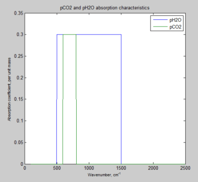
The absorption characteristics for the four model runs:
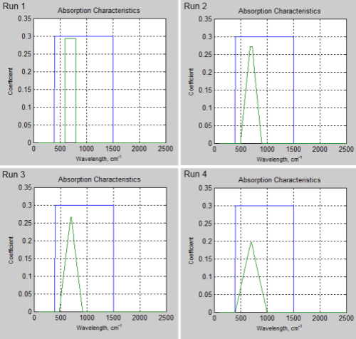
Figure 1 – Blue is pH2O absorption, Green is pCO2 absorption

What happens is that the total band absorptance (the area under the curve) is the same for each run. The pCO2 absorption profile in Run 1 is the same as in all the previous articles in the series. Then in subsequent runs the edges of the band are widened, the “top” is made thinner, and the peak value is adjusted to keep the “total band absorptance” the same.

The code in the notes is specifically for Run 4. The code has to slightly change for each run, as I am changing the shape of the band in each run.

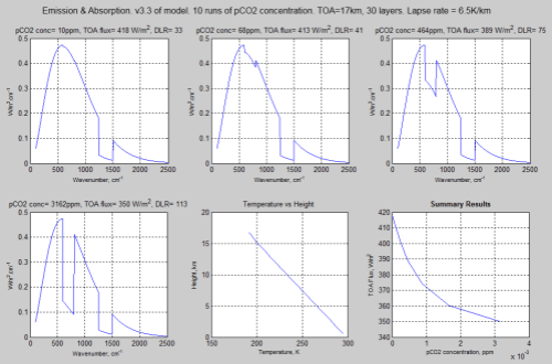
Each model run simulates 20 different pCO2 concentrations. The TOA spectrum for a few results is shown, along with temperature profile, absorption characteristics and the summary of TOA flux vs pCO2 concentration.

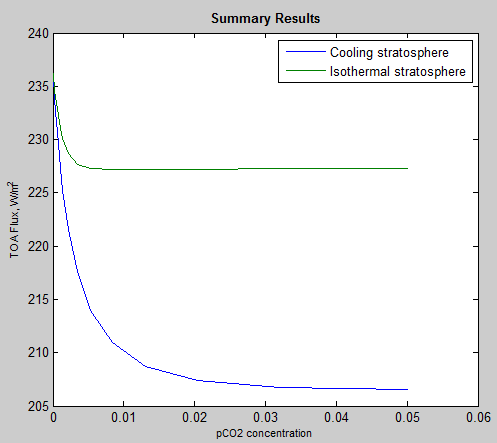
The stratospheric temperature is fixed at 215K – to understand why I’ve chosen to fix it, see the discussion in Part Five.

Run 1:
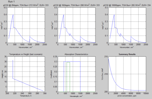
Figure 2 – Click on the image for a larger view

Run 2:

Figure 3 – Click on the image for a larger view

Run 3:
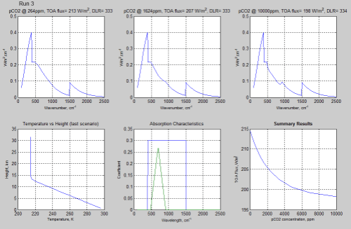
Figure 4 – Click on the image for a larger view

Run 4:
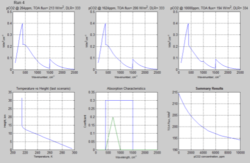
Figure 5 – Click on the image for a larger view

Now let’s compare the summary results from each of the four models:
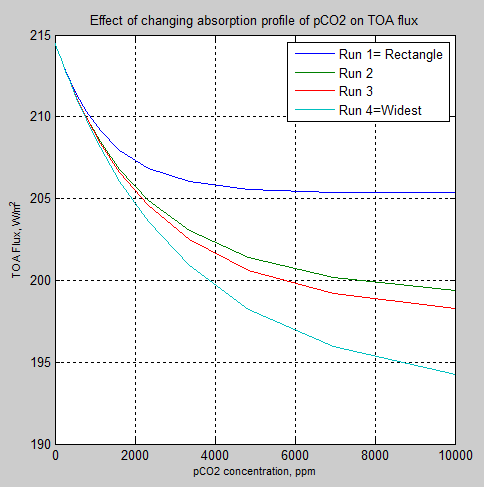
Figure 6 – Changes in TOA flux

And also a reminder that as the TOA flux reduces, the radiative forcing increases – because a reduction in TOA flux means less energy radiated from the planet, and therefore (all other things being equal) a heating effect.

So if we plot the results as radiative forcing instead:
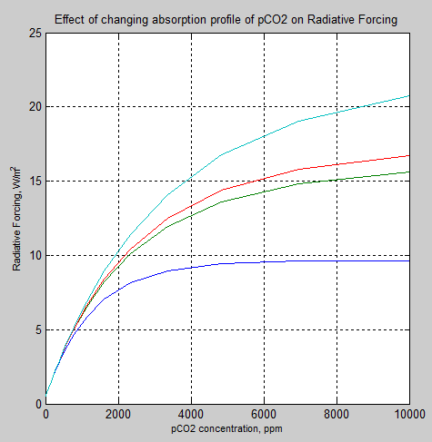
Figure 7 – Radiative Forcing

Effect of Band Shape

The reason for adding this complexity to the model is because real CO2 has an absorption band which is not “rectangular”. The band has a peak absorption around 667 cm-1 (15 μm) which then falls off on either side.

In the results up until now we have seen that different effects contribute to the eventual “saturation” of increasing pCO2 . The particular conditions determine where that saturation takes place.

What these results show is that with a “rectangular” absorption profile the “saturation” takes place much sooner than with a wider band.

Perhaps that is not very surprising to many people.

If it is surprising, then for a conceptual model think about a very strong, very narrow band reaching saturation quite quickly. Whereas if you spread the same absorption over a wider band then each wavelength/wavenumber can contribute more as each wavelength takes longer to reach saturation.

I find it hard to write a good conceptual explanation. Perhaps better to suggest that readers who find the results surprising to reread Part Two to Part Five and review the results from each of the models.

Logarithmic Slopes

I also played around with a logarithmic fall-off instead of a straight line slope. The results were very similar but not identical. I applied the same normalization to the area under the curve as in the previous models.

For example, Run 8, which is similar to Run 4 (similar in that the wavenumbers for the zero points and the “flat top” are identical):
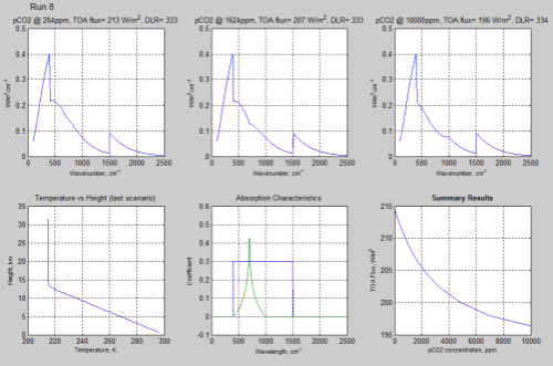
Figure 8 – Click on the image for a larger view

The value of TOA flux at the highest pCO2 concentration of Run 8 was 196.3 W/m², compared with 194.3 W/m² in Run 4.

As less absorption has been “moved out” to the “wings” of the band we would expect that the logarithmic slopes have slightly less effect than the straight line slopes.

Reducing pH2O Effectiveness

I also tried halving the absorption characteristics of pH2O to see the effect. Runs 1-4 were repeated as Runs 9-12 with the only change being the halving of the absorption coefficient of pH2O:
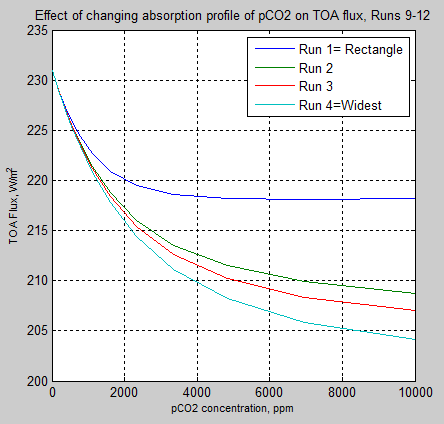
Figure 9

Of course, the total TOA flux is higher in all cases – as pH2O’s effectiveness has been reduced. If you compare the results with Figure 6 you see that curves are quite similar.

Conclusion

Most of the ideas that people have about “saturation” of CO2 are based on a very limited appreciation of how radiative transfer takes place.

The fact that CO2 has very strong absorption in the central part of its band has led to a false conclusion that, therefore, more CO2 can have no further effect.

As we have seen in Part Three, just considering the basic fact of emission totally changes that perspective.

Then we see the effects of emitting from different heights in the atmosphere, and how changing temperature profiles (Part Four) affects that emission.

Another area of confusion is with the idea that because water vapor has absorption across the CO2 band and because water vapor has a much higher concentration than CO2 in the lower troposphere, therefore there is nothing more for CO2 to affect. We saw in Part Four that even making the absorption coefficient of pH2O the same as pCO2  – so that the DLR (back radiation) results were swamped from pH2O – even then the TOA flux was considerably affected by increasing concentrations of pCO2. And in the real world, the real water vapor molecule has considerably less absorption than CO2 around the 15 μm / 667 cm-1 band.

Finally we have seen how a band with a different shape causes quite different results – having a “spreading band” more like the real-world molecules also increases the effect of pCO2 at higher concentrations (less “saturation”).

Well, these are all “model results”

Which means they are the solution to some mathematical equations. If the equations are wrong, then the model is wrong (and if the model writer and his huge team made a mistake in implementation, this model is also wrong).

Yet most of the criticism of “the standard results” in the literature (and as reported by the IPCC) only shows that the critics don’t even know what the equations are.

The usual “explanations” of why the standard results are wrong fall into two categories:

  1. The writers don’t state and solve the radiative transfer equations (see Part Six), but solve something else entirely. They don’t critique the standard equations, a necessary step to demonstrate the standard theory wrong. Going out on a limb, I would say that they don’t know what the standard theory is.
  2. The writers create poetic words with no equations, or happily state one particular fact or figure as a breathless QED. For example, the relative concentration of water vapor vs CO2, the fact that 95% of surface radiation is absorbed within y meters by CO2 at wavelength x.

I hope that most people who have read this series have :

  • a better understanding of how radiative transfer works
  • a vague idea at least of what equations we would expect to see in a successful “critique”
  • an appreciation of how complex the real world is and why a 2 minute calculator result is unlikely to provide insight

There may be more to come from this model. I would like to be able to include some real data on CO2 and play around with it. That might be too much work. You never know until you start.

And of course, requests and suggestions of model results you would like to see are welcome, even if no guarantees are made that the requests will be fulfilled.

Other articles:

Part One – a bit of a re-introduction to the subject.

Part Two – introducing a simple model, with molecules pH2O and pCO2 to demonstrate some basic effects in the atmosphere. This part – absorption only.

Part Three – the simple model extended to emission and absorption, showing what a difference an emitting atmosphere makes. Also very easy to see that the “IPCC logarithmic graph” is not at odds with the Beer-Lambert law.

Part Four – the effect of changing lapse rates (atmospheric temperature profile) and of overlapping the pH2O and pCO2 bands. Why surface radiation is not a mirror image of top of atmosphere radiation.

Part Five – a bit of a wrap up so far as well as an explanation of how the stratospheric temperature profile can affect “saturation”

Part Six – The Equations – the equations of radiative transfer including the plane parallel assumption and it’s nothing to do with blackbodies

Part Seven – changing the shape of the pCO2 band to see how it affects “saturation” – the wings of the band pick up the slack, in a manner of speaking

Part Eight – interesting actual absorption values of CO2 in the atmosphere from Grant Petty’s book

Part Nine – calculations of CO2 transmittance vs wavelength in the atmosphere using the 300,000 absorption lines from the HITRAN database

Part Ten – spectral measurements of radiation from the surface looking up, and from 20km up looking down, in a variety of locations, along with explanations of the characteristics

Part Eleven – Heating Rates – the heating and cooling effect of different “greenhouse” gases at different heights in the atmosphere

Part Twelve – The Curve of Growth – how absorptance increases as path length (or mass of molecules in the path) increases, and how much effect is from the “far wings” of the individual CO2 lines compared with the weaker CO2 lines

And Also –

Theory and Experiment – Atmospheric Radiation – real values of total flux and spectra compared with the theory.

Notes

Note 1: Sharp-eyed observers will eventually point out that I didn’t make use of the diffusivity approximation from Part Six in my model.

Note 2: The Matlab code, v0.5.0

RTE v0.5.0

The code is easiest seen by downloading the word doc, but here it is for reference:

======= v0.5.0 ======================

% RTE = Radiative transfer equations in atmosphere

% Objective – allow progressively more complex applications

% to help people see what happens in practice in the atmosphere

% v0.2 allow iterations of one (or more) parameter to find the TOA flux vs

% changed parameter

% v0.3 add emissivity = absorptivity ; as a function of wavelength. Also

% means that downward and upward radiation must be solved, plus iterations

% to allow temperature to change to find stable solution. Use convective

% adjustment to the lapse rate

% v0.3.1 changes the method of defining the atmosphere layers for radiation

% calculations, to have roughly constant mass for each layer

% v0.3.2 tries changing lapse rates and tropopause heights

% v0.3.3 revises element boundaries as various problems found in testing of

% v0.3.2

% v0.4.0 – introducing overlap of absorption bands

% v0.4.1 – warmer stratosphere to show “saturation” of simple bands

% v0.5.0 – introducing some band “shapes” – instead of just “rectangular”

% absorption bands. pH2O band widened to a min of 400cm^-1

clear  % empty all the variables, so previous runs can have no effect

disp(‘  ‘);

disp([‘—- New Run —- ‘ datestr(now) ‘ —-‘]);

disp(‘  ‘);

% SI units used unless otherwise stated

% ============= Define standard atmosphere against height ================

% first a “high resolution” atmosphere

% zr = height, pr = pressure, Tr = temperature, rhor = density

Ts=300; % define surface temperature

ps=1.013e5; % define surface pressure

Ttropo=215; % define tropopause temperature

% nmv=2.079e25; % nmv x rho = total number of molecules per m^3, not yet

% used

maxzr=50e3; % height of atmosphere

numzr=5001; % number of points used to define real atmosphere

zr=linspace(0,maxzr,numzr); % height vector from sea level to maxzr

[pr Tr rhor ztropo] = define_atmos_0_3(zr,Ts,ps,Ttropo); % function to determine (or lookup) p, T & rho

% Create “coarser resolution” atmosphere – this reduces computation

% requirements for absorption & emission of radiation

% z, p,Tinit,rho; subset of values used for RTE calcs

numz=30; % number of boundaries to consider (number of layers = numz-1)

minp=1e3; % top of atmosphere to consider in pressure (Pa)

% want to divide the atmosphere into approximately equal pressure changes

dp=(pr(1)-minp)/(numz); % finds the pressure change for each height change

zi=zeros(1,numz); % zi = lookup vector to “select” heights, pressures etc

for i=1:numz % locate each value

zi(i)=find(pr<=(pr(1)-i*dp), 1); % gets the location in the vector where

% pressure is that value

end

% now create the vectors of coarser resolution atmosphere

% z(1) = surface; z(numz) = TOA

% T, p, rho all need to be in the midpoint between the boundaries

% T(1) is the temperature between z(1) and z(2), etc.

z=zr(zi);   % height

pb=pr(zi);   % pressure at boundaries

Tb=Tr(zi);   % starting temperature at boundaries

rhob=rhor(zi);  % density at boundaries

% now calculate density, pressure and temperature within each layer

for i=1:numz-1

dz(i)=z(i+1)-z(i); % precalculate thickness of each layer

Tinit(i)=(Tb(i+1)+Tb(i))/2; % temperature in midpoint of boundary

p(i)=(pb(i+1)+pb(i))/2; % pressure in midpoint of boundary

rho(i)=(rhob(i+1)+rhob(i))/2; % density in midpoint of boundary

end

% ============ Set various values =========================

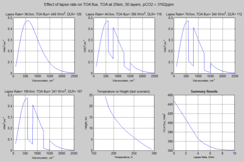
lapse=6.5e-3; % environmental lapse rate in K/m ** note potential conflict with temp profile already determined

% currently = max lapse rate for convective adjustment, but not used to

% define initial temperature profile

ems=0.98; % emissivity of surface

cp=1000; % specific heat capacity of atmosphere, J/K.kg

convadj=true; % === SET TO true === for convective adjustment to lapse rate = lapse

isothermal_strato=true; % ======= SET to true === for fixed and isothermal stratospheric temperature

emission=true; % ==== SET TO true ==== for the atmosphere to emit radiation

tstep=3600*12; % fixed timestep of 1hr

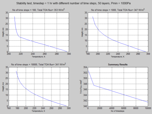
nt=100; % number of timesteps

% work in wavenumber, cm^-1

dv=5;

v=100:dv:2500; % wavenumber (=50um – 4um)

numv=length(v);

rads=ems.*planckmv(v,Ts); % surface emissive spectral power vs wavenumber, v

disp([‘Tstep= ‘ num2str(tstep/3600) ‘ hrs , No of steps= ‘ num2str(nt) ‘, numz= ‘ …

num2str(numz) ‘, minp= ‘ num2str(minp) ‘ Pa, Lapse= ‘ num2str(lapse*1e3) ‘ K/km’]);

% ============== Introducing the molecules ==============================

% need % mixing in the atmosphere vs height, % capture cross section per

% number per frequency, pressure & temperature broadening function

nummol=2; % number of radiatively-active gases

mz=ones(nummol,numz-1); % initialize mixing ratios of the gases

% specific concentrations

% pH2O = pretend H2O

emax=17e-3; % max mixing ratio (surface) of 17g/kg

mz(1,:)=(ztropo-z(1:numz-1)).*emax./ztropo; % straight line reduction from surface to tropopause

mz(1,(mz(1,:)<0))=5e-6; % replace negative values with 5ppm, ie, for heights above tropopause

% pCO2 = pretend CO2

% mz(2,:)=3162e-6; % a fixed mixing ratio for pCO2

% absorption coefficients

k1=0.3; % arbitrary pick – in m2/kg while we use rho

k2=0.3; % likewise

a=zeros(nummol,length(v)); % initialize absorption coefficients

a(1,(v>=400 & v<=1500))=k1;  % wavelength dependent absorption

% define some parameters for the pCO2 band to make it easier to adjust

% and then “normalize” this to the original total band absorptance =

% integral(k.dv) which was 0.3 x 200cm-1 = 60

% note that v1-4 need to be multiples of dv

kint=60; % original total

v2=695;v3=705; % peak “flat top” of band

v1=400;v4=1000; % edges where band absorption coefficient falls to zero

% now optical thickness will fall off as a straight line, later we can try

% transmittance = exp(-tau) falling off as a straight line

% find the location within vector v of these points

vi1=find(v>=v1,1);vi2=find(v>=v2,1);vi3=find(v>=v3,1);vi4=find(v>=v4,1);

a(2,(v>=v2 & v<=v3))=k2;    % flat top of band

for i=vi1:vi2           % rising edge of band

a(2,i)=(v(i)-v1)/(v2-v1)*k2;

end

for i=vi3:vi4        % falling edge of band

a(2,i)=(v4-v(i))/(v4-v3)*k2;

end

knint=sum(a(2,:))*dv; % this adjusts the whole band absorption to make the

% integral the same as the original

a(2,:)=a(2,:)*kint/knint;

disp([‘v1-4= ‘ num2str(v1) ‘, ‘ num2str(v2) ‘, ‘ num2str(v3) ‘, ‘ num2str(v4) ‘, total abs for pCO2 = ‘ num2str(sum(a(2,:))*dv)]);

% plot(v,a) % to show absorption characteristics if required

% return  % if want to early for review of absorption plot

% ========== Scenario loop to change key parameter =======================

% for which we want to see the effect

%

nres=20; % number of results to calculate ******

flux=zeros(1,nres); % TOA flux for each change in parameter

fluxd=zeros(1,nres); % DLR for each change in parameter, not really used yet

par=zeros(1,nres); % parameter we will alter

% this section has to be changed depending on the parameter being changed

% now = pCO2 conc.

par=logspace(-5,-2,nres); % values vary from 10^-5 (10ppm) to 10^-2.5 (3200ppm)

% par=1; % kept for when only one value needed

% ================== Define plots required =======================

% last plot = summary but only if nres>1, ie if more than one scenario

% plot before (or last) = temperature profile, if plottemp=true

% plot before then = surface downward radiation

plottemp=true; % === SET TO true === if plot temperature profile at the end

plotdown=false; % ====SET TO true ==== if downward surface radiation required

plotabs=true; % SET TO true ======= if absorption characteristics required

if nres==1   % if only one scenario

plotix=1;  % only one scenario graph to plot

nplot=plottemp+plotdown+plotabs+1;  % number of plots depends on what options chosen

else     % if more than one scenario, user needs to put values below for graphs to plot

plotix=[round(nres/2) round(nres*3/4) nres]; % graphs to plot – “user” selectable

% plotix=[]; % don’t want to plot any scenarios

nplot=length(plotix)+plottemp+plotdown+plotabs+1; % plot the “plotix” graphs plus the summary

% plus the temperature profile plus downward radiation, if required

end

% work out the location of subplots

if nplot==1

subr=1;subc=1;  % 1 row, 1 column

elseif nplot==2

subr=1;subc=2;  % 1 row, 2 columns

elseif nplot==3 || nplot==4

subr=2;subc=2;  % 2 rows, 2 columns

elseif nplot==5 || nplot==6

subr=2;subc=3;  % 2 rows, 3 columns

else

subr=3;subc=3; % 3 rows, 3 columns

end

for n=1:nres  % each complete run with a new parameter to try

% — the line below has to change depending on parameter chosen

% to find what the stability problem is we need to store all of the

% values of T, to check the maths when it goes unstable

mz(2,:)=par(n); % this is for CO2 changes

% lapse=par(n); % this is for lapse rate changes each run

disp([‘Run = ‘ num2str(n)]);

T=zeros(nt,numz-1); % define array to store T for each level and time step

T(1,:)=Tinit;   % load temperature profile for start of scenario

% remove??? T(:,1)=repmat(Ts,nt,1); % set surface temperature as constant for each time step

% First pre-calculate the transmissivity and absorptivity of each layer

% for each wavenumber. This doesn’t change now that depth of each

% layer, number of each absorber and absorption characteristics are

% fixed.

% n = scenario, i = layer, j = wavenumber, k = absorber

trans=zeros(numz-1,numv); abso=zeros(numz-1,numv); % pre-allocate space

for i=1:numz-1   % each layer

for j=1:numv   % each wavenumber interval

trans=1;  % initialize the amount of transmission within the wavenumber interval

for k=1:nummol  % each absorbing molecule

% for each absorber: exp(-density x mixing ratio x

% absorption coefficient x thickness of layer)

trans=trans*exp(-rho(i)*mz(k,i)*a(k,j)*dz(i)); % calculate transmission, = 1- absorption

end

tran(i,j)=trans;  % transmissivity = 0 – 1

abso(i,j)=(1-trans)*emission;  % absorptivity = emissivity = 1-transmissivity

% if emission=false, absorptivity=emissivity=0

end

end

% === Main loops to calculate TOA spectrum & flux =====

% now (v3) considering emission as well, have to find temperature stability

% first, we cycle around to confirm equilibrium temperature is reached

% second, we work through each layer

% third, through each wavenumber

% fourth, through each absorbing molecule

% currently calculating surface radiation absorption up to TOA AND

% downward radiation from TOA (at TOA = 0)

for h=2:nt  % main iterations to achieve equilibrium

radu=zeros(numz,numv); % initialize upward intensity at each boundary and wavenumber

radd=zeros(numz,numv); % initialize downward intensity at each boundary and wavenumber

radu(1,:)=rads;  % upward surface radiation vs wavenumber

radd(end,:)=zeros(1,numv);  % downward radiation at TOA vs wavenumber

% units of radu, radd are W/m^2.cm^-1, i.e., flux per wavenumber

% h = timestep, i = layer, j = wavenumber

% Upward (have to do upward, then downward)

Eabs=zeros(numz-1); % zero the absorbed energy before we start

for i=1:numz-1   % each layer

for j=1:numv   % each wavenumber interval

% first calculate how much of each monochromatic ray is

% transmitted to the next layer

radu(i+1,j)=radu(i,j)*tran(i,j);

% second, add emission at this wavelength:

% planck function at T(i) x emissivity (=absorptivity)

% this function is spectral emissive power (pi x intensity)

radu(i+1,j)=radu(i+1,j)+abso(i,j)*3.7418e-8.*v(j)^3/(exp(v(j)*1.4388/T(h-1,i))-1);

% Change in energy = dI(v) * dv (per second)

% accumulate through each wavenumber

% if the upwards radiation entering the layer is more than

% the upwards radiation leaving the layer, then a heating

Eabs(i)=Eabs(i)+(radu(i,j)-radu(i+1,j))*dv;

end  % each wavenumber interval

end  % each layer

% Downwards (have to do upward, then downward)

for i=numz-1:-1:1   % each layer from the top down

for j=1:numv   % each wavenumber interval

% first, calculate how much of each monochromatic ray is

% transmitted to the next layer, note that the TOA value

% is set to zero at the start

radd(i,j)=radd(i+1,j)*tran(i,j); % attentuation..

% second, calculate how much is emitted at this wavelength,

radd(i,j)=radd(i,j)+abso(i,j)*3.7418e-8.*v(j)^3/(exp(v(j)*1.4388/T(h-1,i))-1); % addition..

% accumulate energy change per second

Eabs(i)=Eabs(i)+(radd(i+1,j)-radd(i,j))*dv;

end  % each wavenumber interval

dT=Eabs(i)*tstep/(cp*rho(i)*dz(i)); % change in temperature = dQ/heat capacity

if isothermal_strato && z(i)>=ztropo  % if we want to keep stratosphere at fixed temperature

T(h,i)=T(h-1,i);

else

T(h,i)=T(h-1,i)+dT; % calculate new temperature

if T(h,i)>500  % Finite Element analysis problem

disp([‘Terminated at n= ‘ num2str(n) ‘, h= ‘ num2str(h) ‘, z(i)= ‘ num2str(z(i)) ‘, i = ‘ num2str(i)]);

disp([‘time = ‘ num2str(h*tstep/3600) ‘ hrs; = ‘ num2str(h*tstep/3600/24) ‘ days’]);

disp(datestr(now));

return

end

end

% need a step to see how close to an equilibrium we are getting

% not yet implemented

end  % each layer

% now need convective adjustment

if convadj==true  % if convective adjustment chosen..

for i=2:numz-1  % go through each layer

if (T(h,i-1)-T(h,i))/dz(i)>lapse  % too cold, convection will readjust

T(h,i)=T(h,i-1)-(dz(i)*lapse); % adjust temperature

end

end

end

end   % iterations to find equilibrium temperature

flux(n)=sum(radu(end,:))*dv;   % calculate the TOA flux

fluxd(n)=sum(radd(1,:))*dv;   % calculate the DLR total

% === Plotting specific results =======

% Decide if and where to plot

ploc=find(plotix==n);  % is this one of the results we want to plot?

if not(isempty(ploc))  % then plot. “Ploc” is the location within all the plots

subplot(subr,subc,ploc),plot(v,radu(end,:))  % plot wavenumber against TOA emissive power

xlabel(‘Wavenumber, cm^-^1′,’FontSize’,8)

ylabel(‘W/m^2.cm^-^1′,’FontSize’,8)

title([‘pCO2 @ ‘ num2str(round(par(n)*1e6)) ‘ppm, TOA flux= ‘ num2str(round(flux(n)))…

‘ W/m^2, DLR= ‘ num2str(round(fluxd(n)))])

% —

%subplot(subr,subc,ploc),plot(T(end,:),z(2:numz)/1000)

%title([‘Lapse Rate ‘ num2str(par(n)*1000) ‘ K/km, Total TOA flux= ‘ num2str(round(flux(n))) ‘ W/m^2’])

%xlabel(‘Temperature, K’,’FontSize’,8)

%ylabel(‘Height, km’,’FontSize’,8)

grid on

end

end   % end of each run with changed parameter to see TOA effect

if plotdown==true  % plot downward surface radiation, if requested

plotloc=nplot-plottemp-plotabs-(nres>1); % get subplot location

subplot(subr,subc,plotloc),plot(v,radd(2,:))  % plot wavenumber against downward emissive power

title([‘Surface Downward, W/m^2.cm^-^1, Total DLR flux= ‘ num2str(round(fluxd(n))) ‘ W/m^2’])

xlabel(‘Wavenumber, cm^-^1′,’FontSize’,8)

ylabel(‘W/m^2.cm^-^1′,’FontSize’,8)

grid on

end

if plottemp==true  % plot temperature profile vs height, if requested

plotloc=nplot-plotabs-(nres>1); % get subplot location

subplot(subr,subc,plotloc),plot(T(end,:),z(2:numz)/1000)

title(‘Temperature vs Height (last scenario)’)

xlabel(‘Temperature, K’,’FontSize’,8)

ylabel(‘Height, km’,’FontSize’,8)

grid on

end

if plotabs==true % plot show absorption characteristics if required

plotloc=nplot-(nres>1); % get subplot location

subplot(subr,subc,plotloc),plot(v,a) %

title(‘Absorption Characteristics’)

xlabel(‘Wavelength, cm^-^1′,’FontSize’,8)

ylabel(‘Coefficient’,’FontSize’,8)

grid on

end

if nres>1 % produce summary plot – TOA flux vs changed parameter

subplot(subr,subc,nplot),plot(par*1e6,flux)

title(‘Summary Results’,’FontWeight’,’Bold’)

ylabel(‘TOA Flux, W/m^2′,’FontSize’,8)

xlabel(‘pCO2 concentration, ppm’,’FontSize’,8) % ==== change label for different scenarios =========

grid on

end

disp([‘—- Complete End —- ‘ datestr(now) ‘ —-‘]);

Read Full Post »
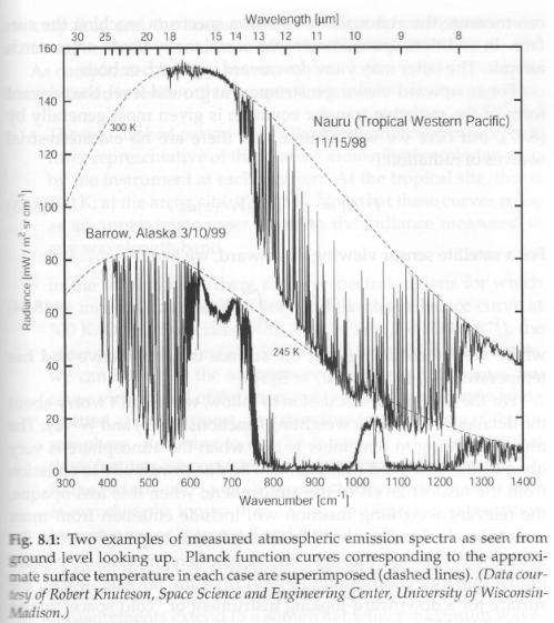
Many blogs write about over-simplifications of the radiative effects in climate. Many of these blog articles review simple explanations of how it is possible for atmospheric radiative effects to increase the surface temperature – e.g. the “blackbody shell” model.

As a result many people are confused and imagine that climate science hasn’t got past “first base” with how radiation interacts with atmospheric gases.

In any field the “over-simplified analysis” is designed to help the beginner to gain conceptual understanding of the field. Not to present the complete field of scientific endeavor.

This article will try to “bridge the gap” between the over-simplified models and the very detailed theory.

Note – it isn’t possible to cover the whole subject in one blog article and a decent treatment of radiative transfer consumes many chapters of a textbook.

There will be some maths. But I will also try to provide a non-mathematical explanation of “the maths” – or “the process”.

If you find maths daunting or incomprehensible that is understandable, but there is a lot that can be learned by trying to grasp some of the basic concepts.

Monochromatic Radiation

This means we need to treat each wavelength separately. Why? Because absorption and emission is a wavelength dependent process.

For example, here is the absorption spectrum of one part of NO2:

From Vardavas & Taylor (2007)

Figure 1

So when we consider radiation “zooming” through the atmosphere we have to take it “one wavelength” at a time.

There isn’t really any such thing as monochromatic radiation or being able to take “one wavelength at a time” – but that doesn’t stop us analyzing the problem..

A Digression on “Calculus”

How does the world of science and engineering deal with continuous change?

If a force, or a ray of radiation, or a movement of the atmosphere is a continuously changing value, how do we define it? How do we deal with it?

Calculus is the answer. This branch of mathematics allows us to deal with small changes and continuous changes and provide theorems, answers and equations.

For example, if we know something about the variable distance, s, with respect to time, t, then an equation defines the relationship between velocity, v, and these other variables:

v = ds/dt

where the “d”s at the beginning means: “the rate of change of”, so the formula means – in English:

Velocity = the rate of change of Distance with respect to Time

Generally when you see something like “da/db” it means “the rate of change of variable a with respect to variable b“.

It is also common to see Δx and δx – meaning “a small change in x”. This is different from “the continuous change of x”, but the specific rationale behind when we use “dx” and “Δx” isn’t so important for this article.

The other important area of calculus is “summing” results when again there is continuous change. If someone travels at 10 km/hr for 1 hour and then at 20km /hr for 1 hr they will have traveled 10km + 20km = 30km. That’s an easy calculation. But if velocity has continuously changed with time – how do we calculate the total distance traveled?

This means, in (harder to understand) English:

Distance = the integral of Velocity with respect to Time, between the limits of time = t1 and time = t2.

The integral is like the summation of each of the tiny distances covered in each very small time period (between t1 and t2). The integral is also often referred to as “the area under the curve”.

..end of digression

Absorption of Radiation

Let’s define a monochromatic beam of radiation, Iλ, travelling through the atmosphere:

Figure 2

We have some information we can use:

The rate of absorption of the beam of radiation as it travels through the atmosphere is proportional to the amount of absorbers at that wavelength and the ability of that absorber to absorb radiation of that wavelength

This is known as the Beer-Lambert law, and is written like this (note 1):

dIλ = -nσIλ .ds       [1]

which means the same thing in mathematical terms, with n=number of absorbing molecules per unit volume (corrected), and σ=capture cross-section (or effectiveness at absorbing at that wavelength), and the subscript λ indicates that this equation is only true for the radiation at this wavelength

The value σ is a material property and so constant for one gas at one wavelength at one temperature and one pressure, but varies with the temperature and pressure of the gas (see comment). The value n will depend on location in the atmosphere. If we solve this equation between two arbitrary points, s1 and s2, we get:

Iλ(s2) = Iλ(s1). exp [ -∫σn(s).ds ]        [2]

where the integral is between the limits s1 and s2

What it means in English:

The intensity of radiation at wavelength λ is reduced as it travels through the atmosphere according to the total amount of the absorber along the path. “exp” is e, or 2.718, to the power of the value in the square brackets.

If the concentration of the gas doesn’t change along the path the equation becomes a simpler version:

Iλ(s2) = Iλ(s1). exp [ -σn.(s2 – s1) ]       [3]

Optical Thickness & Transmittance

These are some important properties to understand.

Optical thickness, usually written as τ, is the property inside the exponential in equation [1].

τ = ∫σn(s).ds         [4]

where the integral is between the limits s1 and s2

Transmittance, usually written with a weird T symbol not available in WordPress, but with “t” here, is the amount of radiation “getting through” along the path we are interested in.

t(s1,s2) = exp [-τ(s1,s2)]       [5]

also written as:

t(s1,s2) = e-τ(s1,s2)

The optical thickness is “dimensionless” as is the transmittance.

So we can rewrite equation [1] as:

Iλ(s2) = Iλ(s1).t(s1,s2)       [6]

The transmittance can be a minimum of zero – although it can never actually get to zero – and a maximum of 1. So it is simply the proportion of radiation at that wavelength which emerges through the section of atmosphere in question:

Figure 3

With optical thickness, τ = 1, transmittance, t = 0.37 – which means that 63% of the radiation is absorbed along the path and 37% is transmitted.

With optical thickness, τ = 10, t=4.5×10⁻⁵ – that is, 45 ppm will be transmitted through the path.

A note on definitions – optical thickness is usually defined as = 0 at the top of atmosphere, where z is a maximum and a maximum at the surface, where z = 0:

Figure 4

So τ increases while z decreases, and z increases while τ decreases.

Absorptance

In the absence of scattering (note 2), absorptance, a = 1 -t.

That is, whatever doesn’t get transmitted gets absorbed.

Plane Parallel Assumption

If you refer back to Figure 2, you see that the radiation is not travelling vertically upwards, but at an angle θ to the vertical.

Using simple trigonometry, ds = dz / cos θ     [7]

It’s always an advantage if we can simplify a problem and relating everything to only the vertical height through the atmosphere helps to solve the equations.

Atmospheric properties vary much more in the vertical direction than in the horizontal direction. For example, go up 10 km and the pressure drops by a factor of 5 – from 1000 mbar to 200 mbar. But travel 10 km horizontally and the pressure will have changed by less than 1 mb. Temperature typically changes 100 times faster in the vertical direction than in the horizontal direction.

And as air density is determined by pressure and absolute temperature we can make a reasonable assumption that the density at a given height, z directly above is the same as the density at the same height when we look at an angle of 45°.

Of course, by the time we are considering an angle close to 90° – i.e., horizontal – the assumption is likely to be invalid. However, the transmissivity of the atmosphere at angles very close to the horizon is extremely low anyway, as we will see.

Therefore, making the assumption of a plane parallel atmosphere is a good approximation.

Let’s review the earlier equations using a mathematical identity that reduces “equation clutter”:

μ = cos θ      [8]

And rewrite equation [5]:

t(z1,z2) = exp [-τ(z1,z2)/μ]       [9]

Notice that the equations are now rewritten in terms of the optical thickness between two vertical heights and the angle of the radiation.

It might help to see it in graphical form – and note here that the optical thickness, τ, is for the vertical direction (otherwise the graph would make no sense):

Figure 5

This simply demonstrates that as the angle increases the radiation has to travel through more atmosphere.

So suppose the optical thickness vertically through the atmosphere, τ = 1, then for:

  • a vertically travelling ray the transmittance = 0.37
  • for a ray at 45° the transmittance = 0.24
  • for a ray at 70° the transmittance = 0.05
  • for a ray at 80° the transmittance = 0.003

Emission

Using Kirchhoff’s law, absorptivity of a material = emissivity of a material for the same wavelength and direction. For diffuse surfaces – and for gases – direction does not affect these material properties, so they are only a function of wavelength. (And for all intents and purposes, absorptance is the same term as absorptivity, and transmittance is the same term as transmissivity-see comment).

Emission of radiation at any given wavelength for a blackbody (a perfect emitter) is given by Planck’s law, which is usually annotated as Bλ(T), where T = temperature.

The absorptivity of a gas, aλ = 1-tλ =emissivity of a gas, ελ.   (Corrected)

For a very small change in monochromatic radiation due to emission:

dIλ = ελBλ(T) .ds        [10a]

Therefore:

dIλ = nσBλ(T) .ds        [10b]

So if now combine emission and absorption, equations 1 & 10:

dI/ds = nσ.(Bλ(T) – Iλ)    [11]

If we combine this with our definition of optical thickness, from equation [4]:

dIλ/dτ = Iλ – Bλ(T)     [12]

which is also known as Schwarzschild’s Equation – and is the fundamental description of changes in radiation as it passes through an absorbing (and non-scattering) atmosphere.

It says, in not so easy to understand English:

The change in monochromatic radiation with respect to optical density is equal to the difference between the intensity of the radiation and the Planck (blackbody) function at the atmospheric temperature

Sorry it’s not clearer in English.

In more vernacular and less precise terms:

As radiation travels through the atmosphere, the intensity increases if the Planck blackbody emission is greater than the incoming radiation and reduces if the Planck blackbody emission is less than the incoming radiation

Solving Schwarzschild’s Equation

Notice that this important equation contains the Planck term, which is for blackbody radiation (i.e., radiation from a perfect emitter), yet the atmosphere is not a perfect emitter. We definitely haven’t assumed that the atmosphere is a blackbody and yet the Planck terms appears in the equation. It’s just how the equation “pans out”..

I mention this only because so many people have come to believe that there is some “big blackbody assumption” in climate science and they might be concerned by this term. Nothing to worry about, this has not been assumed.

Let’s find a solution to the equation if we are measuring the TOA (top of atmosphere) radiation. Refer to Figure 4:

  • at TOA, z=zm and τ=0
  • at the surface, z=0 and τ = τm

Now some maths manipulation – skip to the end people who don’t like maths..

First we note a handy party piece:

d/dτ [Ie] = e. dI/dτ – Ie[13]

Now we multiply both sides of equation [12] by e:

e.dIλ/dτ = e.Iλ – e.Bλ(T)       [14]

Re-arranging:

e.dIλ/dτ – e.Iλ = – e.Bλ(T)       [14a]

And substituting “handy party piece” [13] into [14a]:

d/dτ [Iλe] = – e.Bλ(T)      [15]

Now we integrate [15] between τ=0 and τ=τm:

Iλm)em – Iλ(0) = – ∫ Bλ(T)e dτ    [16]

where the integral is between the limits of 0 and τm

And re-arranging we get:

..end of maths manipulation

Iλ(0) = Iλm)em + ∫ Bλ(T)e dτ    [16]

Which – for those who haven’t followed the intense maths:

Iλ(0) = Iλm)em + ∫ Bλ(T)e [16]

The intensity at the top of atmosphere equals..

The surface radiation attenuated by the transmittance of the atmosphere, plus..

The sum of all the contributions of atmospheric radiation – each contribution attenuated by the transmittance from that location to the top of atmosphere

Don’t worry about the maths, but it is definitely worth spending some time thinking about the words in colors – to get a conceptual understanding of how atmospheric radiation “works”.

It’s Not Over Yet – Conversion from Intensity to Flux and the Diffusivity Approximation

Remember the note about the Plane Parallel Assumption ?

Getting equations into WordPress is painful and time-consuming so a quick explanation followed by the result, especially as maths fatigue will have set in among most readers, if any made it this far.

Equation [16] is for spectral intensity. That is, one direction rather than the complete hemispherical power (flux).

To calculate spectral emissive power (flux per unit wavelength) we need to integrate the equation over one hemisphere of solid angle. We re-write equation [16] in the form of equation [9] so that the optical thickness references vertical height, z and μ, which is the cosine of the angle from the vertical. Then we integrate from μ=0 (θ=0°) to μ=1 (θ=90°).

Transmittance, t(z,0) = 2 ∫ e-τ(z,0)/μ μ.dμ

where the integral is from 0 to 1

This equation doesn’t have an “analytical” solution, meaning we can’t rewrite it in a nice equation form without the integral. But with some clever maths that I haven’t tried to follow – but have checked – we can produce an approximation which is known as the diffusivity approximation:

2 ∫ e-τ(z,0)/μ μ.dμ ≈ e-τ/μ’

Where μ’ is the “effective angle” which produces a close approximation to the actual answer without needing to integrate across all angles (for each wavelength). The best value of μ’ = 0.6.

Here is the calculated integral (left side of the equation) vs the approximation with μ’ = 0.6, as a function of optical thickness, τ, demonstrating the usefulness of the approximation:

Figure 6

There are some other refinements needed, for example, the reflection of atmospheric radiation for a surface emissivity < 1, which is then attenuated by the absorptance of the atmosphere before contributing the TOA measurement. But these factors can all be introduced into the equations.

Full Color Solution

What we have produced so far is a solution for each monochromatic wavelength, λ.

Also, we haven’t explicitly stated the fact that the optical thickness depends on the concentration and “capture cross section” of each absorber for that wavelength. So the optical thickness, and transmittance, for each height requires combining the effects of each active molecule.

The solution for flux, W/m², requires integrating the equations across all wavelengths.

Wow. Conceptually straightforward. But computationally very expensive – check out Figure 1 – the absorption characteristics of each radiatively-active gas vary significantly with wavelength.

Conclusion

The equation for radiative transfer is commonly known, (in differential form) as Schwarzschild’s Equation. It relies on fundamental physics.

To solve the equation requires some maths.

To solve the equation in practical terms the plane parallel assumption is used. This relies on the fact that variations in temperature and pressure (and therefore density) are negligible in the horizontal direction compared with the vertical direction.

The equation could be solved without this plane parallel assumption, but the variations horizontally in pressure and temperature are so slight that the same result would be obtained, unless extremely high quality data on temperature, pressure, density and concentration of absorbers was available.

To solve the equation in practical terms we need to know:

  • the temperature (vs height) in the atmosphere
  • the concentration of each absorber vs height
  • the absorption characteristics of each absorber vs wavelength

In any practical field, the “proof of the pudding is in the eating”, and so take a look at Theory and Experiment – Atmospheric Radiation – where theoretical and practical results are compared.

And lastly, the Stefan-Boltzmann equation, correct and accurate though it is (check out Planck, Stefan-Boltzmann, Kirchhoff and LTE) is not used in the actual equations of radiative transfer in the atmosphere. Nor is any assumption of “unrealistic blackbodies”.

I only note these last points due to the high quantity (but not high quality), of blog articles and comments demonstrating the writers haven’t actually read a textbook on the subject, but still feel qualified to pass judgement on this field of scientific endeavor.

Other articles:

Part One – a bit of a re-introduction to the subject

Part Two – introducing a simple model, with molecules pH2O and pCO2 to demonstrate some basic effects in the atmosphere. This part – absorption only

Part Three – the simple model extended to emission and absorption, showing what a difference an emitting atmosphere makes. Also very easy to see that the “IPCC logarithmic graph” is not at odds with the Beer-Lambert law.

Part Four – the effect of changing lapse rates (atmospheric temperature profile) and of overlapping the pH2O and pCO2 bands. Why surface radiation is not a mirror image of top of atmosphere radiation.

Part Five – a bit of a wrap up so far as well as an explanation of how the stratospheric temperature profile can affect “saturation”

Part Seven – changing the shape of the pCO2 band to see how it affects “saturation” – the wings of the band pick up the slack, in a manner of speaking

And Also –

Theory and Experiment – Atmospheric Radiation – real values of total flux and spectra compared with the theory.

Notes

Note 1: There are many formulations of the Beer-Lambert law and even much dispute about who exactly the law should be attributed to.

Other formulations include using the density of the gas and a matching coefficient for the effectiveness of the gas at absorbing.

Note 2: When considering solar radiation (shortwave), scattering is important. When considering terrestrial radiation (longwave), scattering can be neglected. In this article, we will ignore scattering, so the results will be appropriate for longwave but not correct for shortwave.

Read Full Post »

In Part Four we took a first look at overlapping gases. pH2O’s absorption band was changed to overlap pCO2’s absorption band. And remember that pH2O has a much higher concentration in the lower atmosphere.

For those who haven’t followed the series so far, these are fictional molecules with only a passing resemblance to the real molecules H2O and CO2. The massive complexity of real spectral absorption and emission makes it difficult for people to appreciate the key points of radiative transfer in the atmosphere.

And of course, many people don’t want to “just accept” the results of a hugely complex computer model..

The simple model results revealed some interesting points:

  1. With overlapping bands, increases in pCO2 still led to a reduction in TOA flux.
  2. With increasing pCO2, DLR (back radiation) remains constant and yet TOA flux reduces.

It’s important to understand these results, because it’s very common to see an implicit belief that the TOA results are some kind of “mirror image” of the surface downward results. They aren’t even though of course they are related.

For the results shown in Figure 7 of Part Four, here is the last TOA spectrum and below, the corresponding DLR spectrum:

Figure 1

The balance of energy at TOA is what determines whether the planet warms or cools. Therefore, the spectral values at the surface are not the most important for determining which gases make the most contribution to the inappropriately-named “greenhouse” effect.

And the total value of back radiation at the surface is not what determines the long term surface temperature – because it is possible to reduce the TOA flux without increasing the surface downward flux. (Note 1)

Hopefully, this simple model demonstrates those points clearly.

Just for reference I have added this model version, v0.4.0 to the notes.

Stratospheric Temperatures and “Saturation”

The model results shown in Figure 7 of Part Four show that the TOA flux continues to reduce as the pCO2 concentration increases.

There is an important point here for the ever popular theme of “saturation”.

Let’s take a look at that model again, this time up to very high concentrations of pCO2:

Figure 2 – Click for a larger image

Notice that even as the pCO2 concentration has reached 50,000ppm the TOA flux is still reducing for increasing pCO2.

Also notice the temperature profile (5th graph in figure 2) – it’s important.

Now here is a similar model run with a slightly different constraint:

Figure 3 – Click for a larger image

These results show that “saturation” is reached much sooner. Notice the temperature profile.

The intensity of radiation is dependent on the temperature of the atmosphere from where the radiation takes place.

So if we have an atmosphere that keeps reducing in temperature as we go higher, then no matter how much the concentration of a “greenhouse” gas increases, the ever-higher radiation will be from a colder temperature – and therefore, will keep reducing in intensity.

Of course, eventually the atmosphere thins out to the point where even this effect disappears.

But hopefully the basic physics behind that idea is clear.

This is why in Figure 3 where the stratospheric temperature is held constant and isothermal (all at the same temperature), the changes in TOA flux level off much sooner. No matter where in the stratosphere the atmosphere radiates from it will be at the same temperature. (See the section “Why the Lapse Rate Matters” in Part Four which is covering a very similar point).

Here is the comparison, of 20 different pCO2 concentrations, where the stratosphere was held at 215K (isothermal) and where the stratospheric temperature was allowed to change according to the radiative heating/cooling:

Log plot

Linear plot

The temperature profile of the atmosphere does affect the “saturation” or not question by “greenhouse” gases.

Note that this model is still very simplistic – both of the gases have a fixed absorption within a band and zero outside. Real gases are much more complex and these complexities are very significant in the “saturation” question.

Conclusion

This article is more of a summary and consolidation so far, than any new ideas.

The next article, before covering line width issues, will cover some of the basic maths (and an explanation of the maths) behind how radiation moves through the atmosphere. At least that’s the intent at the moment.

Other articles:

Part One – a bit of a re-introduction to the subject

Part Two – introducing a simple model, with molecules pH2O and pCO2 to demonstrate some basic effects in the atmosphere. This part – absorption only

Part Three – the simple model extended to emission and absorption, showing what a difference an emitting atmosphere makes. Also very easy to see that the “IPCC logarithmic graph” is not at odds with the Beer-Lambert law.

Part Four – the effect of changing lapse rates (atmospheric temperature profile) and of overlapping the pH2O and pCO2 bands. Why surface radiation is not a mirror image of top of atmosphere radiation.

Part Six – The Equations – the equations of radiative transfer including the plane parallel assumption and it’s nothing to do with blackbodies

Part Seven – changing the shape of the pCO2 band to see how it affects “saturation” – the wings of the band pick up the slack, in a manner of speaking

And Also –

Theory and Experiment – Atmospheric Radiation – real values of total flux and spectra compared with the theory.

Notes

Note 1: Reducing the TOA flux = less heat leaves the planet = the planet warms; all other things being equal. More about this idea in The Earth’s Energy Budget – Part Three.

In an immediate sense the back radiation is one of the mechanisms by which the surface is at the temperature it is.

Think of the TOA flux as determining the long term temperature of the surface, and the back radiation as determining the current temperature of the surface.

And for the many who think that this means I am saying convection is unimportant, no I am not. I am explaining one effect on the surface temperature. The essence of understanding a complex subject is to be able to understand the separate effects, and then how they fit together.

Note 2: The Matlab code, v0.4.0:

RTE v0.4.0

The code is easiest seen by downloading the word doc, but here it is for reference:

======= v0.4.0 ======================

% RTE = Radiative transfer equations in atmosphere

% Objective – allow progressively more complex applications

% to help people see what happens in practice in the atmosphere

% v0.2 allow iterations of one (or more) parameter to find the TOA flux vs

% changed parameter

% v0.3 add emissivity = absorptivity ; as a function of wavelength. Also

% means that downward and upward radiation must be solved, plus iterations

% to allow temperature to change to find stable solution. Use convective

% adjustment to the lapse rate

% v0.3.1 changes the method of defining the atmosphere layers for radiation

% calculations, to have roughly constant mass for each layer

% v0.3.2 tries changing lapse rates and tropopause heights

% v0.3.3 revises element boundaries as various problems found in testing of

% v0.3.2

% v0.4.0 – introducing overlap of absorption bands

clear  % empty all the variables, so previous runs can have no effect

disp(‘  ‘);

disp([‘—- New Run —- ‘ datestr(now) ‘ —-‘]);

disp(‘  ‘);

% SI units used unless otherwise stated

% ============= Define standard atmosphere against height ================

% first a “high resolution” atmosphere

% zr = height, pr = pressure, Tr = temperature, rhor = density

Ts=300; % define surface temperature

ps=1.013e5; % define surface pressure

% nmv=2.079e25; % nmv x rho = total number of molecules per m^3, not yet

% used

maxzr=50e3; % height of atmosphere

numzr=5001; % number of points used to define real atmosphere

zr=linspace(0,maxzr,numzr); % height vector from sea level to maxzr

[pr Tr rhor ztropo] = define_atmos_0_2(zr,Ts,ps); % function to determine (or lookup) p, T & rho

% Create “coarser resolution” atmosphere – this reduces computation

% requirements for absorption & emission of radiation

% z, p,Tinit,rho; subset of values used for RTE calcs

numz=30; % number of boundaries to consider (number of layers = numz-1)

minp=3e3; % top of atmosphere to consider in pressure (Pa)

% want to divide the atmosphere into approximately equal pressure changes

dp=(pr(1)-minp)/(numz); % finds the pressure change for each height change

zi=zeros(1,numz); % zi = lookup vector to “select” heights, pressures etc

for i=1:numz % locate each value

zi(i)=find(pr<=(pr(1)-i*dp), 1); % gets the location in the vector where

% pressure is that value

end

% now create the vectors of coarser resolution atmosphere

% z(1) = surface; z(numz) = TOA

% T, p, rho all need to be in the midpoint between the boundaries

% T(1) is the temperature between z(1) and z(2), etc.

z=zr(zi);   % height

pb=pr(zi);   % pressure at boundaries

Tb=Tr(zi);   % starting temperature at boundaries

rhob=rhor(zi);  % density at boundaries

% now calculate density, pressure and temperature within each layer

for i=1:numz-1

dz(i)=z(i+1)-z(i); % precalculate thickness of each layer

Tinit(i)=(Tb(i+1)+Tb(i))/2; % temperature in midpoint of boundary

p(i)=(pb(i+1)+pb(i))/2; % pressure in midpoint of boundary

rho(i)=(rhob(i+1)+rhob(i))/2; % density in midpoint of boundary

end

% ============ Set various values =========================

lapse=6.5e-3; % environmental lapse rate in K/m ** note potential conflict with temp profile already determined

% currently = max lapse rate for convective adjustment, but not used to

% define initial temperature profile

ems=0.98; % emissivity of surface

cp=1000; % specific heat capacity of atmosphere, J/K.kg

convadj=true; % === SET TO true === for convective adjustment to lapse rate = lapse

emission=true; % ==== SET TO true ==== for the atmosphere to emit radiation

tstep=3600*12; % fixed timestep of 1hr

nt=1000; % number of timesteps

% work in wavenumber, cm^-1

dv=5;

v=100:dv:2500; % wavenumber (=50um – 4um)

numv=length(v);

rads=ems.*planckmv(v,Ts); % surface emissive spectral power vs wavenumber, v

disp([‘Tstep= ‘ num2str(tstep/3600) ‘ hrs , No of steps= ‘ num2str(nt) ‘, numz= ‘ …

num2str(numz) ‘, minp= ‘ num2str(minp) ‘ Pa, Lapse= ‘ num2str(lapse*1e3) ‘ K/km’]);

% ============== Introducing the molecules ==============================

% need % mixing in the atmosphere vs height, % capture cross section per

% number per frequency, pressure & temperature broadening function

nummol=2; % number of radiatively-active gases

mz=ones(nummol,numz-1); % initialize mixing ratios of the gases

% specific concentrations

% pH2O = pretend H2O

emax=17e-3; % max mixing ratio (surface) of 17g/kg

mz(1,:)=(ztropo-z(1:numz-1)).*emax./ztropo; % straight line reduction from surface to tropopause

mz(1,(mz(1,:)<0))=5e-6; % replace negative values with 5ppm, ie, for heights above tropopause

% pCO2 = pretend CO2

mz(2,:)=3162e-6; % a fixed mixing ratio for pCO2

% absorption coefficients

k1=0.3; % arbitrary pick – in m2/kg while we use rho

k2=0.3; % likewise

a=zeros(nummol,length(v)); % initialize absorption coefficients

a(1,(v>=500 & v<=1500))=k1;  % wavelength dependent absorption

a(2,(v>=600 & v<=800))=k2;    % ” ”

% ========== Scenario loop to change key parameter =======================

% for which we want to see the effect

%

nres=10; % number of results to calculate ******

flux=zeros(1,nres); % TOA flux for each change in parameter

fluxd=zeros(1,nres); % DLR for each change in parameter, not really used yet

par=zeros(1,nres); % parameter we will alter

% this section has to be changed depending on the parameter being changed

% now = pCO2 conc.

par=logspace(-5,-2.5,nres); % values vary from 10^-5 (10ppm) to 10^-2.5 (3200ppm)

% par=1; % kept for when only one value needed

% ================== Define plots required =======================

% last plot = summary but only if nres>1, ie if more than one scenario

% plot before (or last) = temperature profile, if plottemp=true

% plot before then = surface downward radiation

plottemp=false; % === SET TO true === if plot temperature profile at the end

plotdown=true; % ====SET TO true ==== if downward surface radiation required

if nres==1   % if only one scenario

plotix=1;  % only one scenario graph to plot

nplot=plottemp+plotdown+1;  % number of plots depends on what options chosen

else     % if more than one scenario, user needs to put values below for graphs to plot

plotix=[1 round(nres/2) 8 nres]; % graphs to plot – “user” selectable

nplot=length(plotix)+plottemp+plotdown+1; % plot the “plotix” graphs plus the summary

% plus the temperature profile plus downward radiation, if required

end

% work out the location of subplots

if nplot==1

subr=1;subc=1;  % 1 row, 1 column

elseif nplot==2

subr=1;subc=2;  % 1 row, 2 columns

elseif nplot==3 || nplot==4

subr=2;subc=2;  % 2 rows, 2 columns

elseif nplot==5 || nplot==6

subr=2;subc=3;  % 2 rows, 3 columns

else

subr=3;subc=3; % 3 rows, 3 columns

end

for n=1:nres  % each complete run with a new parameter to try

% — the line below has to change depending on parameter chosen

% to find what the stability problem is we need to store all of the

% values of T, to check the maths when it goes unstable

mz(2,:)=par(n); % this is for CO2 changes

% lapse=par(n); % this is for lapse rate changes each run

disp([‘Run = ‘ num2str(n)]);

T=zeros(nt,numz-1); % define array to store T for each level and time step

T(1,:)=Tinit;   % load temperature profile for start of scenario

% remove??? T(:,1)=repmat(Ts,nt,1); % set surface temperature as constant for each time step

% First pre-calculate the transmissivity and absorptivity of each layer

% for each wavenumber. This doesn’t change now that depth of each

% layer, number of each absorber and absorption characteristics are

% fixed.

% n = scenario, i = layer, j = wavenumber, k = absorber

trans=zeros(numz-1,numv); abso=zeros(numz-1,numv); % pre-allocate space

for i=1:numz-1   % each layer

for j=1:numv   % each wavenumber interval

trans=1;  % initialize the amount of transmission within the wavenumber interval

for k=1:nummol  % each absorbing molecule

% for each absorber: exp(-density x mixing ratio x

% absorption coefficient x thickness of layer)

trans=trans*exp(-rho(i)*mz(k,i)*a(k,j)*dz(i)); % calculate transmission, = 1- absorption

end

tran(i,j)=trans;  % transmissivity = 0 – 1

abso(i,j)=(1-trans)*emission;  % absorptivity = emissivity = 1-transmissivity

% if emission=false, absorptivity=emissivity=0

end

end

% === Main loops to calculate TOA spectrum & flux =====

% now (v3) considering emission as well, have to find temperature stability

% first, we cycle around to confirm equilibrium temperature is reached

% second, we work through each layer

% third, through each wavenumber

% fourth, through each absorbing molecule

% currently calculating surface radiation absorption up to TOA AND

% downward radiation from TOA (at TOA = 0)

for h=2:nt  % main iterations to achieve equilibrium

radu=zeros(numz,numv); % initialize upward intensity at each boundary and wavenumber

radd=zeros(numz,numv); % initialize downward intensity at each boundary and wavenumber

radu(1,:)=rads;  % upward surface radiation vs wavenumber

radd(end,:)=zeros(1,numv);  % downward radiation at TOA vs wavenumber

% units of radu, radd are W/m^2.cm^-1, i.e., flux per wavenumber

% h = timestep, i = layer, j = wavenumber

% Upward (have to do upward, then downward)

Eabs=zeros(numz-1); % zero the absorbed energy before we start

for i=1:numz-1   % each layer

for j=1:numv   % each wavenumber interval

% first calculate how much of each monochromatic ray is

% transmitted to the next layer

radu(i+1,j)=radu(i,j)*tran(i,j);

% second, add emission at this wavelength:

% planck function at T(i) x emissivity (=absorptivity)

% this function is spectral emissive power (pi x intensity)

radu(i+1,j)=radu(i+1,j)+abso(i,j)*3.7418e-8.*v(j)^3/(exp(v(j)*1.4388/T(h-1,i))-1);

% Change in energy = dI(v) * dv (per second)

% accumulate through each wavenumber

% if the upwards radiation entering the layer is more than

% the upwards radiation leaving the layer, then a heating

Eabs(i)=Eabs(i)+(radu(i,j)-radu(i+1,j))*dv;

end  % each wavenumber interval

end  % each layer

% Downwards (have to do upward, then downward)

for i=numz-1:-1:1   % each layer from the top down

for j=1:numv   % each wavenumber interval

% first, calculate how much of each monochromatic ray is

% transmitted to the next layer, note that the TOA value

% is set to zero at the start

radd(i,j)=radd(i+1,j)*tran(i,j); % attentuation..

% second, calculate how much is emitted at this wavelength,

radd(i,j)=radd(i,j)+abso(i,j)*3.7418e-8.*v(j)^3/(exp(v(j)*1.4388/T(h-1,i))-1); % addition..

% accumulate energy change per second

Eabs(i)=Eabs(i)+(radd(i+1,j)-radd(i,j))*dv;

end  % each wavenumber interval

dT=Eabs(i)*tstep/(cp*rho(i)*dz(i)); % change in temperature = dQ/heat capacity

T(h,i)=T(h-1,i)+dT; % calculate new temperature

if T(h,i)>500  % Finite Element analysis problem

disp([‘Terminated at n= ‘ num2str(n) ‘, h= ‘ num2str(h) ‘, z(i)= ‘ num2str(z(i)) ‘, i = ‘ num2str(i)]);

disp([‘time = ‘ num2str(h*tstep/3600) ‘ hrs; = ‘ num2str(h*tstep/3600/24) ‘ days’]);

disp(datestr(now));

return

end

% need a step to see how close to an equilibrium we are getting

% not yet implemented

end  % each layer

% now need convective adjustment

if convadj==true  % if convective adjustment chosen..

for i=2:numz-1  % go through each layer

if (T(h,i-1)-T(h,i))/dz(i)>lapse  % too cold, convection will readjust

T(h,i)=T(h,i-1)-(dz(i)*lapse); % adjust temperature

end

end

end

end   % iterations to find equilibrium temperature

flux(n)=sum(radu(end,:))*dv;   % calculate the TOA flux

fluxd(n)=sum(radd(1,:))*dv;   % calculate the DLR total

% === Plotting specific results =======

% Decide if and where to plot

ploc=find(plotix==n);  % is this one of the results we want to plot?

if not(isempty(ploc))  % then plot. “Ploc” is the location within all the plots

subplot(subr,subc,ploc),plot(v,radu(end,:))  % plot wavenumber against TOA emissive power

xlabel(‘Wavenumber, cm^-^1′,’FontSize’,8)

ylabel(‘W/m^2.cm^-^1′,’FontSize’,8)

title([‘pCO2 @ ‘ num2str(round(par(n)*1e6)) ‘ppm, TOA flux= ‘ num2str(round(flux(n)))…

‘ W/m^2, DLR= ‘ num2str(round(fluxd(n)))])

% —

%subplot(subr,subc,ploc),plot(T(end,:),z(2:numz)/1000)

%title([‘Lapse Rate ‘ num2str(par(n)*1000) ‘ K/km, Total TOA flux= ‘ num2str(round(flux(n))) ‘ W/m^2’])

%xlabel(‘Temperature, K’,’FontSize’,8)

%ylabel(‘Height, km’,’FontSize’,8)

grid on

end

end   % end of each run with changed parameter to see TOA effect

if plotdown==1  % plot downward surface radiation, if requested

plotloc=nplot-plottemp-(nres>1); % get subplot location

subplot(subr,subc,plotloc),plot(v,radd(2,:))  % plot wavenumber against downward emissive power

title([‘Surface Downward, W/m^2.cm^-^1, Total DLR flux= ‘ num2str(round(fluxd(n))) ‘ W/m^2’])

xlabel(‘Wavenumber, cm^-^1′,’FontSize’,8)

ylabel(‘W/m^2.cm^-^1′,’FontSize’,8)

grid on

end

if plottemp==1  % plot temperature profile vs height, if requested

plotloc=nplot-(nres>1); % get subplot location

subplot(subr,subc,plotloc),plot(T(end,:),z(2:numz)/1000)

title(‘Temperature vs Height (last scenario)’)

xlabel(‘Temperature, K’,’FontSize’,8)

ylabel(‘Height, km’,’FontSize’,8)

grid on

end

if nres>1 % produce summary plot – TOA flux vs changed parameter

subplot(subr,subc,nplot),plot(par*1e6,flux)

title(‘Summary Results’,’FontWeight’,’Bold’)

ylabel(‘TOA Flux, W/m^2′,’FontSize’,8)

xlabel(‘pCO2 concentration, ppm’,’FontSize’,8) % ==== change label for different scenarios =========

grid on

end

disp([‘—- Complete End —- ‘ datestr(now) ‘ —-‘]);

Read Full Post »
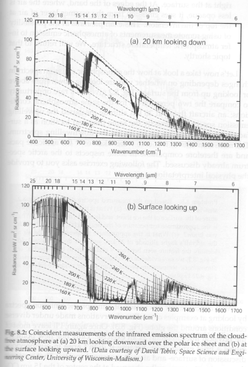
In Part Three we saw some results of absorption and emission in the atmosphere but later I commented that the model had some flaws.

Take a look at Part Three for more about the model.

The Model Flaws and Update

The model (v0.3.1) had poorly defined boundaries and as a result the downward flux through a layer of the atmosphere was affecting the temperature of an adjacent layer.

I noticed the problems when looking at the model stratospheric temperature profile (the upper atmosphere). According to theory, with no ozone the stratospheric temperature shouldn’t increase from the tropopause. Yet in my model it did. So I ran some stability tests:

  • different number of layers
  • different top of atmosphere height/pressure
  • longer runs
  • shorter and longer time steps

Flaws kept appearing, including instabilities.

Anyway, the model is now fixed (according to the army of Science of Doom testers). v0.3.3 is logged in the notes.

Because the flaw was in the stratosphere, fixing the flaw (luckily) had minimal effect on the TOA flux results previously reported. Here are the new results:

Figure 1 – Click on image for a larger view

Note: ppm concentration in “Summary Results” has an incorrect legend. It is not ppm, but just a mixing ratio. The highest value is just over 3×10⁻³ , i.e., just over 3000 ppm.

If we compare with Figure 2 in Part Three, we see the results are similar.

Here are some stability test results after the model was fixed, trying different time steps for the same total time, and comparing the final temperature profile as well as TOA flux:

Figure 2 – Click on image for a larger view

Note: there is an error in the graph title. The model time period was 10,000 hrs (60 weeks).

And trying a fixed time step with different number of timesteps (so the total time is variable):

Figure 3 – Click on image for a larger view

So with the earlier mistakes out of the way..

Why the Lapse Rate Matters

Here are the results from 8 runs with fixed pCO2 concentration (at the highest value from earlier runs) and different lapse rates (note 1). Only 4 of the individual results are shown, and the temperature profile is from the last run:

Figure 4 – Click on image for a larger view

The first graph shows that the TOA flux is equal to the surface flux – and the spectrum shows no characteristic “notches” in it. Yet there are 2 highly absorbing gases (pH2O and pCO2) present. How can this be?

The radiatively-active gases absorb and also emit. If the emission is from a location in the atmosphere which is at the same temperature as the source of the original radiation then, in simple terms, “the amount taken out (absorbed)” = “the amount put back in (emitted)”.

The lapse rate increases in each of the following 3 graphs in figure 4, meaning that the atmosphere gets colder at any given height. Therefore, the emitted radiation from a given height will be from a colder gas and therefore will be of a lower intensity.

Questionif the lapse rate in the last scenario run is 10 K/km what do we learn from the 5th graph, which shows temperature vs height?

What the above model runs show is that changes in the lapse rate affect the inappropriately-named “greenhouse” effect = the difference between the surface radiation and the TOA radiation.

For example, if there is more water vapor in the lower atmosphere the lapse rate will reduce. As a result the TOA flux will increase. And, as already explained in Part Three (under “Reducing Emission and “The Greenhouse Effect”), this will have the effect of reducing the surface temperature – all other things being equal. Of course, more water vapor will also change the atmospheric absorption so all other things aren’t equal.

Overlapping Bands

A common area of concern for people trying to understand the effect of absorbing gases in the atmosphere is this:

How can CO2 have any impact when water vapor has a much higher concentration in the lower atmosphere, has such a high absorption and overlaps the CO2 band?

The model results might be interesting here. The model is still very simplistic. Here are the new absorption characteristics:

Figure 5

For no particular reason the absorption coefficients are the same, and the pH2O absorption now completely encompasses the pCO2 band.

As in Part Two, the concentration of pH2O in the lower atmosphere is much higher than pCO2, even for the highest concentration of pCO2 simulated:

Figure 6

Here are the results of the simulation runs:

Figure 7 – Click on the image for a larger view

This should be of interest. pH2O has a much higher concentration in the lower atmosphere. Yet, as the concentration of pCO2 increases the TOA flux is affected significantly. Of course, not nearly as much as when pCO2 alone affected 600-800 cm-1, and the concentration has to reach a higher value than before to affect the TOA flux.

Notice as well that the DLR, or back radiation, is constant in each of the graphs in the last figure. How can this be?

Plenty of food for thought.

Last point for reference – these are fictional molecules, created for the purpose of illustrating the effect of absorption and emission through the atmosphere. They have vaguely similar characteristics to the real molecules H2O and CO2, but are far from identical.

Conclusion

The simplistic model demonstrates that lapse rate plays an important part in the effect on top of atmosphere fluxes.

The model also demonstrates that even with a higher concentration absorber in the lower atmosphere, an absorber higher up in the atmosphere can have a significant effect.

These kind of results are not easy to calculate in your head. That’s just because the equations of radiative transfer, although well-known, are not linear. And not many people can calculate summations – in their head – across multiple changing variables when one of the key terms is e-x.

The model is still quite simple, not including effects like line width and its dependence on pressure and temperature. And not including the hideous complexity that is stored in the HITRANS database.

Other articles:

Part One – a bit of a re-introduction to the subject

Part Two – introducing a simple model, with molecules pH2O and pCO2 to demonstrate some basic effects in the atmosphere. This part – absorption only

Part Three – the simple model extended to emission and absorption, showing what a difference an emitting atmosphere makes. Also very easy to see that the “IPCC logarithmic graph” is not at odds with the Beer-Lambert law.

Part Five – a bit of a wrap up so far as well as an explanation of how the stratospheric temperature profile can affect “saturation”

Part Six – The Equations – the equations of radiative transfer including the plane parallel assumption and it’s nothing to do with blackbodies

Part Seven – changing the shape of the pCO2 band to see how it affects “saturation” – the wings of the band pick up the slack, in a manner of speaking

And Also –

Theory and Experiment – Atmospheric Radiation – real values of total flux and spectra compared with the theory.


Notes

Note 1: Lapse rate is the temperature change with altitude – typically a reduction of 6.5K per km. This is primarily governed by “adiabatic expansion” and is affected by the amount of water vapor in the atmosphere. See Venusian Mysteries and the following articles for more.

Note 2: The Matlab code, v0.3.3

RTE v0.3.3

The code is easiest seen by downloading the word doc, but here it is for reference:

======= v0.3.3 ======================

% RTE = Radiative transfer equations in atmosphere

% Objective – allow progressively more complex applications

% to help people see what happens in practice in the atmosphere

% v0.2 allow iterations of one (or more) parameter to find the TOA flux vs

% changed parameter

% v0.3 add emissivity = absorptivity ; as a function of wavelength. Also

% means that downward and upward radiation must be solved, plus iterations

% to allow temperature to change to find stable solution. Use convective

% adjustment to the lapse rate

% v0.3.1 changes the method of defining the atmosphere layers for radiation

% calculations, to have roughly constant mass for each layer

% v0.3.2 tries changing lapse rates and tropopause heights

% v0.3.3 revises element boundaries as various problems found in testing of

% v0.3.2

clear  % empty all the variables, so previous runs can have no effect

disp(‘  ‘);

disp([‘—- New Run —- ‘ datestr(now) ‘ —-‘]);

disp(‘  ‘);

% SI units used unless otherwise stated

% ============= Define standard atmosphere against height ================

% first a “high resolution” atmosphere

% zr = height, pr = pressure, Tr = temperature, rhor = density

Ts=300; % define surface temperature

ps=1.013e5; % define surface pressure

% nmv=2.079e25; % nmv x rho = total number of molecules per m^3, not yet

% used

maxzr=50e3; % height of atmosphere

numzr=5001; % number of points used to define real atmosphere

zr=linspace(0,maxzr,numzr); % height vector from sea level to maxzr

[pr Tr rhor ztropo] = define_atmos_0_2(zr,Ts,ps); % function to determine (or lookup) p, T & rho

% Create “coarser resolution” atmosphere – this reduces computation

% requirements for absorption & emission of radiation

% z, p,Tinit,rho; subset of values used for RTE calcs

numz=30; % number of boundaries to consider (number of layers = numz-1)

minp=1e4; % top of atmosphere to consider in pressure (Pa)

% want to divide the atmosphere into approximately equal pressure changes

dp=(pr(1)-minp)/(numz); % finds the pressure change for each height change

zi=zeros(1,numz); % zi = lookup vector to “select” heights, pressures etc

for i=1:numz % locate each value

zi(i)=find(pr<=(pr(1)-i*dp), 1); % gets the location in the vector where

% pressure is that value

end

% now create the vectors of coarser resolution atmosphere

% z(1) = surface; z(numz) = TOA

% T, p, rho all need to be in the midpoint between the boundaries

% T(1) is the temperature between z(1) and z(2), etc.

z=zr(zi);   % height

pb=pr(zi);   % pressure at boundaries

Tb=Tr(zi);   % starting temperature at boundaries

rhob=rhor(zi);  % density at boundaries

% now calculate density, pressure and temperature within each layer

for i=1:numz-1

dz(i)=z(i+1)-z(i); % precalculate thickness of each layer

Tinit(i)=(Tb(i+1)+Tb(i))/2; % temperature in midpoint of boundary

p(i)=(pb(i+1)+pb(i))/2; % pressure in midpoint of boundary

rho(i)=(rhob(i+1)+rhob(i))/2; % density in midpoint of boundary

end

% ============ Set various values =========================

lapse=6.5e-3; % environmental lapse rate in K/m ** note potential conflict with temp profile already determined

% currently = max lapse rate for convective adjustment, but not used to

% define initial temperature profile

ems=0.98; % emissivity of surface

cp=1000; % specific heat capacity of atmosphere, J/K.kg

convadj=true; % === SET TO true === for convective adjustment to lapse rate = lapse

emission=true; % ==== SET TO true ==== for the atmosphere to emit radiation

tstep=3600*12; % fixed timestep of 1hr

nt=1000; % number of timesteps

% work in wavenumber, cm^-1

dv=5;

v=100:dv:2500; % wavenumber (=50um – 4um)

numv=length(v);

rads=ems.*planckmv(v,Ts); % surface emissive spectral power vs wavenumber, v

disp([‘Tstep= ‘ num2str(tstep/3600) ‘hrs , No of steps= ‘ num2str(nt) ‘, numz= ‘ num2str(numz) ‘, minp= ‘ num2str(minp) ‘Pa, lapse= ‘ num2str(lapse*1000) ‘ K/km’]);

% ============== Introducing the molecules ==============================

% need % mixing in the atmosphere vs height, % capture cross section per

% number per frequency, pressure & temperature broadening function

nummol=2; % number of radiatively-active gases

mz=ones(nummol,numz-1); % initialize mixing ratios of the gases

% specific concentrations

% pH2O = pretend H2O

emax=17e-3; % max mixing ratio (surface) of 17g/kg

mz(1,:)=(ztropo-z(1:numz-1)).*emax./ztropo; % straight line reduction from surface to tropopause

mz(1,(mz(1,:)<0))=5e-6; % replace negative values with 5ppm, ie, for heights above tropopause

% pCO2 = pretend CO2

mz(2,:)=3e-3; % a fixed mixing ratio for pCO2

% absorption coefficients

k1=0.3; % arbitrary pick – in m2/kg while we use rho

k2=0.3; % likewise

a=zeros(nummol,length(v)); % initialize absorption coefficients

a(1,(v>=1250 & v<=1500))=k1;  % wavelength dependent absorption

a(2,(v>=600 & v<=800))=k2;    % ” ”

% ========== Scenario loop to change key parameter =======================

% for which we want to see the effect

%

nres=10; % number of results to calculate ******

flux=zeros(1,nres); % TOA flux for each change in parameter

fluxd=zeros(1,nres); % DLR for each change in parameter, not really used yet

par=zeros(1,nres); % parameter we will alter

% this section has to be changed depending on the parameter being changed

% now = CO2 concentration

par=logspace(-5,-2.5,nres); % values vary from 10^-5 (10ppm) to 10^-2.5 (3200ppm)

% par=1; % kept for when only one value needed

% ================== Define plots required =======================

% last plot = summary but only if nres>1, ie if more than one scenario

% plot before (or last) = temperature profile, if plottemp=true

% plot before then = surface downward radiation

plottemp=true; % === SET TO true === if plot temperature profile at the end

plotdown=false; % ====SET TO true ==== if downward surface radiation required

if nres==1   % if only one scenario

plotix=1;  % only one scenario graph to plot

nplot=plottemp+plotdown+1;  % number of plots depends on what options chosen

else     % if more than one scenario, user needs to put values below for graphs to plot

plotix=[1 4 7 nres]; % graphs to plot – “user” selectable

nplot=length(plotix)+plottemp+plotdown+1; % plot the “plotix” graphs plus the summary

% plus the temperature profile plus downward radiation, if required

end

% work out the location of subplots

if nplot==1

subr=1;subc=1;  % 1 row, 1 column

elseif nplot==2

subr=1;subc=2;  % 1 row, 2 columns

elseif nplot==3 || nplot==4

subr=2;subc=2;  % 2 rows, 2 columns

elseif nplot==5 || nplot==6

subr=2;subc=3;  % 2 rows, 3 columns

else

subr=3;subc=3; % 3 rows, 3 columns

end

for n=1:nres  % each complete run with a new parameter to try

% — the line below has to change depending on parameter chosen

% to find what the stability problem is we need to store all of the

% values of T, to check the maths when it goes unstable

mz(2,:)=par(n);

disp([‘Run = ‘ num2str(n)]);

T=zeros(nt,numz-1); % define array to store T for each level and time step

T(1,:)=Tinit;   % load temperature profile for start of scenario

% remove??? T(:,1)=repmat(Ts,nt,1); % set surface temperature as constant for each time step

% First pre-calculate the transmissivity and absorptivity of each layer

% for each wavenumber. This doesn’t change now that depth of each

% layer, number of each absorber and absorption characteristics are

% fixed.

% n = scenario, i = layer, j = wavenumber, k = absorber

trans=zeros(numz-1,numv); abso=zeros(numz-1,numv); % pre-allocate space

for i=1:numz-1   % each layer

for j=1:numv   % each wavenumber interval

trans=1;  % initialize the amount of transmission within the wavenumber interval

for k=1:nummol  % each absorbing molecule

% for each absorber: exp(-density x mixing ratio x

% absorption coefficient x thickness of layer)

trans=trans*exp(-rho(i)*mz(k,i)*a(k,j)*dz(i)); % calculate transmission, = 1- absorption

end

tran(i,j)=trans;  % transmissivity = 0 – 1

abso(i,j)=(1-trans)*emission;  % absorptivity = emissivity = 1-transmissivity

% if emission=false, absorptivity=emissivity=0

end

end

% === Main loops to calculate TOA spectrum & flux =====

% now (v3) considering emission as well, have to find temperature stability

% first, we cycle around to confirm equilibrium temperature is reached

% second, we work through each layer

% third, through each wavenumber

% fourth, through each absorbing molecule

% currently calculating surface radiation absorption up to TOA AND

% downward radiation from TOA (at TOA = 0)

for h=2:nt  % main iterations to achieve equilibrium

radu=zeros(numz,numv); % initialize upward intensity at each boundary and wavenumber

radd=zeros(numz,numv); % initialize downward intensity at each boundary and wavenumber

radu(1,:)=rads;  % upward surface radiation vs wavenumber

radd(end,:)=zeros(1,numv);  % downward radiation at TOA vs wavenumber

% units of radu, radd are W/m^2.cm^-1, i.e., flux per wavenumber

% h = timestep, i = layer, j = wavenumber

% Upward (have to do upward, then downward)

Eabs=zeros(numz-1); % zero the absorbed energy before we start

for i=1:numz-1   % each layer

for j=1:numv   % each wavenumber interval

% first calculate how much of each monochromatic ray is

% transmitted to the next layer

radu(i+1,j)=radu(i,j)*tran(i,j);

% second, add emission at this wavelength:

% planck function at T(i) x emissivity (=absorptivity)

% this function is spectral emissive power (pi x intensity)

radu(i+1,j)=radu(i+1,j)+abso(i,j)*3.7418e-8.*v(j)^3/(exp(v(j)*1.4388/T(h-1,i))-1);

% Change in energy = dI(v) * dv (per second)

% accumulate through each wavenumber

% if the upwards radiation entering the layer is more than

% the upwards radiation leaving the layer, then a heating

Eabs(i)=Eabs(i)+(radu(i,j)-radu(i+1,j))*dv;

end  % each wavenumber interval

end  % each layer

% Downwards (have to do upward, then downward)

for i=numz-1:-1:1   % each layer from the top down

for j=1:numv   % each wavenumber interval

% first, calculate how much of each monochromatic ray is

% transmitted to the next layer, note that the TOA value

% is set to zero at the start

radd(i,j)=radd(i+1,j)*tran(i,j); % attentuation..

% second, calculate how much is emitted at this wavelength,

radd(i,j)=radd(i,j)+abso(i,j)*3.7418e-8.*v(j)^3/(exp(v(j)*1.4388/T(h-1,i))-1); % addition..

% accumulate energy change per second

Eabs(i)=Eabs(i)+(radd(i+1,j)-radd(i,j))*dv;

end  % each wavenumber interval

dT=Eabs(i)*tstep/(cp*rho(i)*dz(i)); % change in temperature = dQ/heat capacity

T(h,i)=T(h-1,i)+dT; % calculate new temperature

if T(h,i)>500  % Finite Element analysis problem

disp([‘Terminated at n= ‘ num2str(n) ‘, h= ‘ num2str(h) ‘, z(i)= ‘ num2str(z(i)) ‘, i = ‘ num2str(i)]);

disp([‘time = ‘ num2str(h*tstep/3600) ‘ hrs; = ‘ num2str(h*tstep/3600/24) ‘ days’]);

disp(datestr(now));

return

end

% need a step to see how close to an equilibrium we are getting

% not yet implemented

end  % each layer

% now need convective adjustment

if convadj==true  % if convective adjustment chosen..

for i=2:numz-1  % go through each layer

if (T(h,i-1)-T(h,i))/dz(i)>lapse  % too cold, convection will readjust

T(h,i)=T(h,i-1)-(dz(i)*lapse); % adjust temperature

end

end

end

end   % iterations to find equilibrium temperature

flux(n)=sum(radu(end,:))*dv;   % calculate the TOA flux

fluxd(n)=sum(radd(1,:))*dv;   % calculate the DLR total

% === Plotting specific results =======

% Decide if and where to plot

ploc=find(plotix==n);  % is this one of the results we want to plot?

if not(isempty(ploc))  % then plot. “Ploc” is the location within all the plots

subplot(subr,subc,ploc),plot(v,radu(end,:))  % plot wavenumber against TOA emissive power

xlabel(‘Wavenumber, cm^-^1′,’FontSize’,8)

ylabel(‘W/m^2.cm^-^1′,’FontSize’,8)

title([‘pCO2 conc= ‘ num2str(round(par(n)*1e6)) ‘ppm, TOA flux= ‘ num2str(round(flux(n)))…

‘ W/m^2, DLR= ‘ num2str(round(fluxd(n)))])

% —

% subplot(subr,subc,ploc),plot(T(end,:),z(2:numz)/1000)

% title([‘No of time steps = ‘ num2str(par(n)) ‘, Total TOA flux= ‘ num2str(round(flux(n))) ‘ W/m^2’])

% xlabel(‘Temperature, K’,’FontSize’,8)

% ylabel(‘Height, km’,’FontSize’,8)

grid on

end

end   % end of each run with changed parameter to see TOA effect

if plotdown==1  % plot downward surface radiation, if requested

plotloc=nplot-plottemp-(nres>1); % get subplot location

subplot(subr,subc,plotloc),plot(v,radd(2,:))  % plot wavenumber against downward emissive power

title([‘Surface Downward, W/m^2.cm^-^1, Total DLR flux= ‘ num2str(round(fluxd(n))) ‘ W/m^2’])

xlabel(‘Wavenumber, cm^-^1′,’FontSize’,8)

ylabel(‘W/m^2.cm^-^1′,’FontSize’,8)

grid on

end

if plottemp==1  % plot temperature profile vs height, if requested

plotloc=nplot-(nres>1); % get subplot location

subplot(subr,subc,plotloc),plot(T(end,:),z(2:numz)/1000)

title(‘Temperature vs Height’)

xlabel(‘Temperature, K’,’FontSize’,8)

ylabel(‘Height, km’,’FontSize’,8)

grid on

end

if nres>1 % produce summary plot – TOA flux vs changed parameter

subplot(subr,subc,nplot),plot(par,flux)

title(‘Summary Results’,’FontWeight’,’Bold’)

ylabel(‘TOA Flux, W/m^2′,’FontSize’,8)

xlabel(‘pCO2 concentration, ppm’,’FontSize’,8) % ==== change label for different scenarios =========

grid on

end

disp([‘—- Complete End —- ‘ datestr(now) ‘ —-‘]);

Read Full Post »
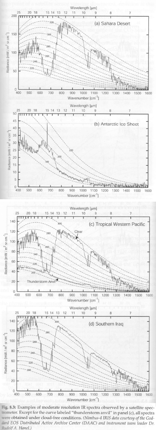
In Part Two, we looked at the beginnings of a very simple 1-d model for examining how the atmosphere interacts with radiation from the surface.

Simplification aids understanding so the model has some fictious gases which absorb radiation – pCO2 (pretend CO2) and pH2O (pretend water vapor). We saw that as the concentrations of pCO2 were increased we stopped seeing a change in “top of atmosphere” (TOA) flux.

That is, the “greenhouse” effect became “saturated” as the pCO2 concentration was increased.

Of course, the model was flawed. The model only included absorption of radiation by the atmosphere, with no emission. There are other over-simplifications and progressively we will try and consider them.

Emission

Once the atmosphere can emit as well as absorb radiation the results change.

The model has been updated, and for these results is now at v3.1 (see note 5).

Here is a comparison of “no emission” vs “emission”. In each case 10 runs were carried out of different pCO2 concentrations. Each graph shows:

  • TOA spectral results for runs 1, 5 and 10
  • Surface spectral downward radiation (DLR or “back radiation) for the last run
  • Temperature profile for the last run
  • Summary graph of flux vs concentration changes for all 10 runs

No emission:

Figure 1 – Click for a larger view

Note that the surface downward radiation is zero. This is because the atmosphere doesn’t emit radiation in this model.

With emission:

Figure 2 – Click for a larger image

If you compare the spectral results you can see that in the “no emission” case the “pretend water vapor” (pH2O) band of wavenumbers 1250-1500 cm-1 is in “saturation”, whereas in the “emission” case, it isn’t.

This is just the natural result of an atmosphere that re-emits – and of course, gases that absorb at a given wavelength also emit at that same wavelength. (See Planck, Stefan-Boltzmann, Kirchhoff and LTE).

And a comparison of the 10 runs between the two models:

Figure 3

As the concentration of pCO2 increases the TOA flux reduces. Of course, we can see that this effect diminishes with more pCO2.

One interesting idea is to show these results as radiative forcing. (You can find a more formal definition of the term in CO2 – An Insignificant Trace Gas? Part Seven – The Boring Numbers – although here it is not calculated according to the strict definition of allowing stratospheric adjustment)

In essence radiative forcing is the change in TOA flux. When less flux escapes this is considered a positive radiative forcing. The reason is this: less flux radiated from the climate system means that less energy is leaving, which means the climate will heat (all other things being equal).

Here is the same graph expressed as radiative forcing:

Figure 4

If you compare it with the IPCC graph in Part Two (or Part Seven of the CO2 series) you will see it has some similarities:

Figure 5

Note that the actual values of radiative forcing in this model are much higher – in part because we are comparing the results of a gas with made up properties and also because we are comparing the effect from ZERO concentration of the gas vs a very high concentration.

However, one point should be clear. Using the very simple Beer-Lambert law of absorption, and the very well-known (but not so simple) Planck law of emission we find that the “radiative forcing” for changing concentrations of one gas doesn’t look like the Beer-Lambert law of absorption..

Real World Complexity

The very simple model here – with emission – will eventually reach “saturation”.

The much more complex real-world “line by line” models eventually reach “saturation” but at much higher concentrations of CO2 than we expect to see in the climate.

This model is still a very simple model designed for education of the basics – and to allow inspection of the code.

The model has no overlaps between absorbing molecules and has no effects from the weaker lines at the edges of a band.

Reducing Emission and “The Greenhouse Effect”

As emission of radiation is reduced due to increases in absorbing gases, with all other things being equal, the planet must warm up. It must warm up until the emission of radiation again balances the absorbed radiation (note 1).

Another way to consider the effect is to think about where the radiation to space comes from in the atmosphere. As the opacity of the atmosphere increases the radiation to space must be from a higher altitude. See also The Earth’s Energy Budget – Part Three.

Higher altitudes are colder and so the radiation to space is a lower value. Less radiation from the climate means the climate warms.

As the climate warms, if the lapse rate (note 3) stays the same, eventually the radiation to space – from this higher altitude – will match the absorbed solar radiation. This is how increases in radiatively active gases (aka “greenhouse” gases) affect the surface temperature (see note 4).

The Model

The equations will be covered more thoroughly in a later article in this series.

The essence of the model is captured in this diagram for one “layer”:

Figure 6 – One layer from the model

The atmosphere is broken up into a number of layers. In these model runs this was set to 30 layers with a minimum pressure of 10,000 Pa (about 17km). The “boundary condition” for radiation from the surface was Planck law radiation from a surface of 300K (27°C) with an emissivity of 0.98. And the “boundary condition” for radiation from TOA was zero.

This is because we are considering “longwave radiation”. A further complication would be to consider an absorber (like CO2) which absorbs solar radiation, but this has not been done in this model. Absorbers of “shortwave” radiation trap energy in the atmosphere rather than allowing it to be absorbed at the surface. Therefore, they affect the “in planetary balance” but don’t significantly affect the total energy absorbed.

The transmissivity at each wavenumber for each layer was calculated. Absorptivity = 1- transmissivity (note 2).

So for each layer – and each wavenumber interval – the transmitted radiation (incident radiation x transmissivity) was calculated for each wavenumber. This was done separately for up and down radiation. The emitted radiation was calculated by the Planck formula and the emissivity (= absorptivity at that wavenumber).

The net energy absorbed as a result changed the temperature, and the model iterated through many time steps to find the final result.

With the very simple pCO2 and pH2O properties the number of timesteps made almost no difference to the TOA flux. The stratospheric temperature did vary, something for further investigation.

The wavenumber interval, dv = 5cm-1, was changed to see the results. Very small changes were observed as dv changed from 5cm-1 to 1cm-1. This is not surprising as the absorbing properties of these molecules is very simple.

Conclusion

The model is still very simple.

The changes in TOA fluxes are significantly different for the unrealistic “no emission” case vs the “emission” case. This is to be expected.

As concentration of pCO2 increases the TOA flux reduces but by progressively smaller amounts.

When we review the results as “radiative forcing” we find that even with this simple model they resemble the IPCC “logarithmic forcing result”.

There’s more to think about with real-world gases and absorption.

Hopefully this article helps people who are trying to understand the basics a little better.

And surely there must be mistakes in the code. Anyone who sees anything questionable, please comment. You will probably be correct.

People trying to do these calculations in their head, or with a pocket calculator, will be wrong. Unless they are mathematical savants. Playing the odds here.. when someone says (on this subject): “I can see that …” or “It’s clear that..” without a statement of the radiative transfer equations and boundary conditions plus their solutions to the problem – I expect that they haven’t understood the problem. And mathematical savants still need to explain to rest of us how they reached their results.

Other articles:

Part One – a bit of a re-introduction to the subject

Part Two – introducing a simple model, with molecules pH2O and pCO2 to demonstrate some basic effects in the atmosphere. This part – absorption only

Part Four – the effect of changing lapse rates (atmospheric temperature profile) and of overlapping the pH2O and pCO2 bands. Why surface radiation is not a mirror image of top of atmosphere radiation.

Part Five – a bit of a wrap up so far as well as an explanation of how the stratospheric temperature profile can affect “saturation”

Part Six – The Equations – the equations of radiative transfer including the plane parallel assumption and it’s nothing to do with blackbodies

Part Seven – changing the shape of the pCO2 band to see how it affects “saturation” – the wings of the band pick up the slack, in a manner of speaking

And Also –

Theory and Experiment – Atmospheric Radiation – real values of total flux and spectra compared with the theory.


Notes

Note 1: Simplifications aid understanding. But in the current “climate” where many assume that climate science doesn’t understand complexity it is worth explaining a little further. Words from others neatly describe the subject of “equilibrium”:

The dominant factor determining the surface temperature of a planet is the balance between the net incoming solar radiation and outgoing thermal infra-red radiation.

That is, radiative equilibrium can be assumed for most practical purposes, although strictly speaking it is never achieved, as time-dependent and non-radiative processes are always present..

I.M. Vardavas & Prof. F.W. Taylor, Radiation and Climate, Oxford University Press (2007)

Note 2: Scattering of solar radiation is important, but scattering of longwave (terrestrial radiation) is very small and can be neglected. Therefore, Absorption = 1 – Transmission.

Note 3: Lapse rate is the temperature change with altitude – typically a reduction of 6.5K per km. This is primarily governed by “adiabatic expansion” and is affected by the amount of water vapor in the atmosphere. See Venusian Mysteries and the following articles for more.

Note 4: The explanations here do not include the effects of feedback. Feedback is very important, but separating different effects is important for understanding.

Note 5: The model still has many simplifications. The Matlab code:

RTE v0.3.1

It is easier to read by downloading the word doc. But pasted here below for reference. The two functions called are already documented in Part Two (and have not changed).

Matlab has many great features, but they also mean that some aspects of the code might not be clear. Feel free to ask questions.

I already see that a comment doesn’t match the code. The time step, tstep=3600*3 is 3 hrs not 12 hrs, as the comment says. However, this doesn’t alter the results.

======= v 0.3.1 ================

% RTE = Radiative transfer equations in atmosphere

% Objective – allow progressively more complex applications

% to help people see what happens in practice in the atmosphere

% v0.2 allow iterations of one (or more) parameter to find the TOA flux vs

% changed parameter

% v0.3 add emissivity = absorptivity ; as a function of wavelength. Also

% means that downward and upward radiation must be solved, plus iterations

% to allow temperature to change to find stable solution. Use convective

% adjustment to the lapse rate

% v0.3.1 changes the method of defining the atmosphere layers for radiation

% calculations, to have roughly constant mass for each layer

% Define standard atmosphere against height

% zr = height, pr = pressure, Tr = temperature, rhor = density, all in SI units

Ts=300; % define surface temperature

ps=1.013e5; % define surface pressure

% nmv=2.079e25; % nmv x rho = total number of molecules per m^3, not yet

% used

maxzr=50e3; % height of atmosphere

numzr=2001; % number of points used to define real atmosphere

zr=linspace(0,maxzr,numzr); % height vector from sea level to maxzr

[pr Tr rhor ztropo] = define_atmos(zr,Ts,ps); % function to determine (or lookup) p, T & rho

% Consider atmosphere in a coarser resolution than used for calculating

% pressure, temperature etc

% z, p,T,rho; subset of values used for RTE calcs

numz=30; % number of layers to consider

minp=1e4; % top of atmosphere to consider in pressure (Pa)

% want to divide the atmosphere into equal pressure changes

dp=(pr(1)-minp)/(numz); % finds the pressure change for each height change

zi=zeros(1,numz); % zi = lookup vector to “select” heights, pressures etc

for i=1:numz % locate each value

zi(i)=find(pr<=(pr(1)-i*dp), 1); % gets the location in the vector where

% pressure is that value

end

% now create the vectors of coarser resolution atmosphere

z=zr(zi);   % height

p=pr(zi);   % pressure

T=Tr(zi);   % original temperature

rho=rhor(zi);  % density

for i=2:numz

dz(i)=z(i)-z(i-1); % precalculate thickness of each layer

end

% ============ Set various values =========================

lapse=6.5e-3; % environmental lapse rate in K/m ** note potential conflict with temp profile already determined

% currently = max lapse rate for convective adjustment, but not used to

% define initial temperature profile

ems=0.98; % emissivity of surface

cp=1000; % specific heat capacity of atmosphere, J/K.kg

convadj=true; % === SET TO true === for convective adjustment to lapse rate = lapse

emission=true; % ==== SET TO true ==== for the atmosphere to emit radiation

% work in wavenumber, cm^-1

dv=5;

v=100:dv:2500; % wavenumber (=50um – 4um)

numv=length(v);

rads=ems.*planckmv(v,Ts); % surface emissive spectral power vs wavenumber v

% ============== Introducing the molecules ==============================

% need % mixing in the atmosphere vs height, % capture cross section per

% number per frequency, pressure & temperature broadening function

nummol=2; % number of radiatively-active gases

mz=ones(nummol,numz); % initialize mixing ratios of the gases

% specific concentrations

% pH2O = pretend H2O

emax=17e-3; % max mixing ratio (surface) of 17g/kg

mz(1,:)=(ztropo-z).*emax./ztropo; % straight line reduction from surface to tropopause

mz(1,(mz(1,:)<0))=5e-6; % replace negative values with 5ppm, ie, for heights above tropopause

% pCO2 = pretend CO2

mz(2,:)=3.6e-4; % 360ppm

% absorption coefficients

k1=0.3; % arbitrary pick – in m2/kg while we use rho

k2=0.3; % likewise

a=zeros(nummol,length(v)); % initialize absorption coefficients

a(1,(v>=1250 & v<=1500))=k1;  % wavelength dependent absorption

a(2,(v>=600 & v<=800))=k2;    % ” ”

% === Scenario loop to change key parameter for which we want to see the effect

%

nres=10; % number of results to calculate

flux=zeros(1,nres); % TOA flux for each change in parameter

par=zeros(1,nres); % parameter we will alter

% this section has to be changed depending on the parameter being changed

% now = CO2 concentration

par=logspace(-5,-2.5,nres); % values vary from 10^-5 (10ppm) to 10^-2.5 (3200ppm)

% par=0.01; % kept for when only one value needed

% ================== Define plots required =======================

% last plot = summary but only if nres>1, ie if more than one scenario

% plot before (or last) = temperature profile, if plottemp=true

% plot before then = surface downward radiation

plottemp=true; % === SET TO true === if plot temperature profile at the end

plotdown=true; % ====SET TO true ==== if downward surface radiation required

if nres==1   % if only one scenario

plotix=1;  % only one scenario graph to plot

nplot=plottemp+plotdown+1;  % number of plots depends on what options chosen

else     % if more than one scenario, user needs to put values below for graphs to plot

plotix=[1 round(nres/2) nres]; % graphs to plot – “user” selectable

nplot=length(plotix)+plottemp+plotdown+1; % plot the “plotix” graphs plus the summary

% plus the temperature profile plus downward radiation, if required

end

% work out the location of subplots

if nplot==1

subr=1;subc=1;  % 1 row, 1 column

elseif nplot==2

subr=1;subc=2;  % 1 row, 2 columns

elseif nplot==3 || nplot==4

subr=2;subc=2;  % 2 rows, 2 columns

elseif nplot==5 || nplot==6

subr=2;subc=3;  % 2 rows, 3 columns

else

subr=3;subc=3; % 3 rows, 3 columns

end

for n=1:nres  % each complete run with a new parameter to try

% — the line below has to change depending on parameter chosen

mz(2,:)=par(n);

% First pre-calculate the transmissivity and absorptivity of each layer

% for each wavenumber. This doesn’t change now that depth of each

% layer, number of each absorber and absorption characteristics are

% fixed.

% n = scenario, i = layer, j = wavenumber, k = absorber

trans=zeros(numz,numv); abso=zeros(numz,numv); % pre-allocate space

for i=2:numz   % each layer

for j=1:numv   % each wavenumber interval

trans=1;  % initialize the amount of transmission within the wavenumber interval

for k=1:nummol  % each absorbing molecule

% for each absorber: exp(-density x mixing ratio x

% absorption coefficient x thickness of layer)

trans=trans*exp(-rho(i)*mz(k,i)*a(k,j)*dz(i)); % calculate transmission, = 1- absorption

end

tran(i,j)=trans;  % transmissivity = 0 – 1

abso(i,j)=(1-trans)*emission;  % absorptivity = emissivity = 1-transmissivity

% if emission=false, absorptivity=emissivity=0

end

end

% === Main loops to calculate TOA spectrum & flux =====

% now (v3) considering emission as well, have to find temperature stability

% first, we cycle around to confirm equilibrium temperature is reached

% second, we work through each layer

% third, through each wavenumber

% fourth, through each absorbing molecule

% currently calculating surface radiation absorption up to TOA AND

% downward radiation from TOA (at TOA = 0)

% has temperature changed loop.. not yet written

% not changing pressure and density with temperature changes – only

% minor variation

tstep=3600*3; % each time step in seconds = 12 hour

for h=1:100  % main iterations to achieve equilibrium

radu=zeros(numz,numv); % initialize upward intensity at each height and wavenumber

radd=zeros(numz,numv); % initialize downward intensity at each height and wavenumber

radu(1,:)=rads;  % upward surface radiation vs wavenumber

radd(end,:)=0;  % downward radiation at TOA vs wavenumber

% units of radu, radd are W/m^2.cm^-1, i.e., flux per wavenumber

% h = timestep, i = layer, j = wavenumber

% Upward (have to do upward, then downward)

Eabs=zeros(numz); % zero the absorbed energy before we start

for i=2:numz   % each layer

for j=1:numv   % each wavenumber interval

% first calculate how much of each monochromatic ray is

% transmitted to the next layer

radu(i,j)=radu(i-1,j)*tran(i,j);

% second, calculate how much is emitted at this wavelength,

% planck function at T(i) x emissivity (=absorptivity)

% this function is spectral emissive power (pi x intensity)

radu(i,j)=radu(i,j)+abso(i,j)*3.7418e-8.*v(j)^3/(exp(v(j)*1.4388/T(i))-1);

% Change in energy = dI(v) * dv (per second)

% accumulate through each wavenumber

Eabs(i)=Eabs(i)+(radu(i,j)-radu(i-1,j))*dv;

end  % each wavenumber interval

end  % each layer

% Downards (have to do upward, then downward)

for i=numz-1:-1:2   % each layer from the top down

for j=1:numv   % each wavenumber interval

% first, calculate how much of each monochromatic ray is

% transmitted to the next layer, note that the TOA value

% is set to zero at the start

radd(i,j)=radd(i+1,j)*tran(i,j);

% second, calculate how much is emitted at this wavelength,

radd(i,j)=radd(i,j)+abso(i,j)*3.7418e-8.*v(j)^3/(exp(v(j)*1.4388/T(i))-1);

% accumulate energy change per second

Eabs(i)=Eabs(i)+(radu(i,j)-radu(i-1,j))*dv;

end  % each wavenumber interval

dT=Eabs(i)*tstep/(cp*rho(i)*dz(i)); % change in temperature = dQ/heat capacity

T(i)=T(i)+dT; % calculate new temperature

% need a step to see how close to an equilibrium we are getting

% not yet implemented

end  % each layer

% now need convective adjustment

if convadj==true  % if convective adjustment chosen..

for i=2:numz  % go through each layer

if (T(i-1)-T(i))/dz(i)>lapse  % too cold, convection will readjust

T(i)=T(i-1)-(dz(i)*lapse); % adjust temperature

end

end

end

end   % iterations to find equilibrium temperature

flux(n)=sum(radu(end,:)*dv);   % calculate the TOA flux

% === Plotting specific results =======

% Decide if and where to plot

ploc=find(plotix==n);  % is this one of the results we want to plot?

if not(isempty(ploc))  % then plot. “Ploc” is the location within all the plots

subplot(subr,subc,ploc),plot(v,radu(end,:))  % plot wavenumber against TOA emissive power

xlabel(‘Wavenumber, cm^-^1′,’FontSize’,8)

ylabel(‘W/m^2.cm^-^1′,’FontSize’,8)

title([‘pCO2 = ‘ num2str(round(par(n)*1e6)) ‘ppm, Total TOA flux= ‘ num2str(round(flux(n))) ‘ W/m^2’])

grid on

end

end   % end of each run with changed parameter to see TOA effect

if plotdown==1  % plot downward surface radiation, if requested

plotloc=nplot-plottemp-(nres>1); % get subplot location

subplot(subr,subc,plotloc),plot(v,radd(2,:))  % plot wavenumber against downward emissive power

title(‘Surface Downward, W/m^2.cm^-^1’)

xlabel(‘Wavenumber, cm^-^1′,’FontSize’,8)

ylabel(‘W/m^2.cm^-^1′,’FontSize’,8)

grid on

end

if plottemp==1  % plot temperature profile vs height, if requested

plotloc=nplot-(nres>1); % get subplot location

subplot(subr,subc,plotloc),plot(T,z/1000)

title(‘Temperature vs Height’)

xlabel(‘Temperature, K’,’FontSize’,8)

ylabel(‘Height, km’,’FontSize’,8)

grid on

end

if nres>1 % produce summary plot – TOA flux vs changed parameter

subplot(subr,subc,nplot),plot(par*1e6,flux)

title(‘Summary Results’,’FontWeight’,’Bold’)

ylabel(‘TOA Flux, W/m^2′,’FontSize’,8)

xlabel(‘pCO2 ppm’,’FontSize’,8) % ==== change label for different scenarios =========

grid on

end

Read Full Post »
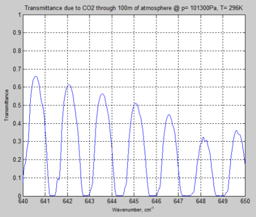
In Part One I said:

In the next part we will consider more advanced aspects of this subject.

However, although that is where we are heading, first I want to look at a very simple model and progressively increase its complexity. It may be illuminating.

The discussions on the Radiative Transfer Equations at the very informative blog of Judith Curry’s were very interesting. Many comments showed an appreciation for the very basics with a misunderstanding of how they fit together, for example:

IPCC declares that infrared absorption is proportional to the logarithm of GHG concentration. It is not. A logarithm might be fit to the actual curve over a small region, but it is not valid for calculations much beyond that region like IPCC’s projections. The physics governing gas absorption is the Beer-Lambert Law, which IPCC never mentions nor uses. The Beer-Lambert Law provides saturation as the gas concentration increases. IPCC’s logarithmic relation never saturates, but quickly gets silly, going out of bounds as it begins its growth to infinity.

There have also been many questions asked at this blog about the various aspects of radiation and atmosphere, so I thought some examples – via a model – might be beneficial.

The Model

The main purpose of this model is to demonstrate the effect of the basic absorption and emission processes on top of atmosphere fluxes. It is not designed to work out what troubles may lie ahead for the climate.

This model is designed to demonstrate some basic ideas about what are known as the radiative transfer equations – how radiation is absorbed and emitted as it travels from the surface to the top of atmosphere (and also from the top of atmosphere to the surface).

I aim to bridge a gap between the “blackbody shell” models and the line-by-line climate models – in a way that people can understand. Ambitious aims.

The advantage of this model should be that we can try different ideas. And the code is available for inspection.

Absorption and Beer-Lambert

The equation of absorption is known as the Beer-Lambert law – you can see more about it in CO2 – An Insignificant Trace Gas? Part Three.

In essence the Beer-Lambert law demonstrates that absorption of radiation of any wavelength is dependent on the amount of the molecule in the path of the radiation & how effective it is at absorbing at that wavelength (note 1):

Figure 1 – Beer-Lambert Law

Simple Model – v0.2 – Saturation

The simple model (v0.2) starts by creating an atmosphere. First of all, atmospheric temperatures, “created”, by definition. Second, using the temperatures plus the hydrostatic equation to calculate the pressure vs height. Third, the density (not shown) is derived.

The surface temperature is 300K.

Figure 2

In this first version of the model (v0.2), we introduce two radiatively-active molecules (=”greenhouse” gases):

  • pH2O – pretend H2O
  • pCO2 – pretend CO2

They have some vague relationship with the real molecules of similar names, but the model objective is simplicity, so of course, these molecules aren’t as complex as the real-life water vapor and CO2. And their absorption characteristics are in no way intended to be the same as the real molecules.

The mixing ratio of pH2O:

Figure 3 – water vapor mixing ratio

The pCO2 mixing ratio is constant with height, but the ppm value is varied from model run to model run.

So onto our top of atmosphere results. I’ll refer to “top of atmosphere” as TOA from now on. These results are at 20km, a fairly arbitrary choice.

The results are shown against wavenumber, which is more usual in spectroscopy, but less easy to visualize than wavelength. Wavenumber = 10,000/wavelength (when wavelength is in μm and wavenumber is in cm-1.

  • 15 μm = 667 cm-1
  • 10 μm = 1,000 cm-1
  • 4 μm = 2,500 cm-1

The “notch” that starts to appear around 600-700 cm-1 is from pCO2 as we increase its concentration. The effect of pH2O is held constant. You can see the effect of pH2O as the “notch” around wavenumbers 1250-1500.

Note that the final graph summarizes the results – TOA Flux vs pCO2 concentration:

Figure 4

What we see is that eventually we reach a point where more pCO2 has no more effect – saturation!

We see that as the concentration keeps on increasing we get a reduction in the TOA flux down to a “saturated” value.

And when we plot the Summary Results we get something that looks very like the Beer-Lambert law of absorption! Nothing like the IPCC result shown in CO2 – An Insignificant Trace Gas? Part Seven – The Boring Numbers:

Radiative Forcing vs CO2 concentration, Myhre et al (1998)

Radiative Forcing vs CO2 concentration, Myhre et al (1998)

Figure 5

So, case closed then?

Flaws in the Model

This model is very simplistic. Most importantly, it only includes absorption of radiation and does not include emission.

Simplifications:

  • no emission from any layers in the atmosphere
  • no dependence of line width on pressure and temperature
  • no weaker “wings” of an absorption band
  • no overlapping of absorption (absorption by 2 molecules in the same band)

In fact, the model only represents the Beer Lambert law of absorption and therefore is incomplete. If the atmosphere is absorbing energy from radiation, where is this energy going?

The next step is to add emission.

Another important point is that the total number of people involved in creating, testing and checking this model = 1.

Surely there will be mistakes.. I welcome comments from sharp-eyed observers pointing out the mistakes.

Other articles:

Part One – a bit of a re-introduction to the subject

Part Three – the simple model extended to emission and absorption, showing what a difference an emitting atmosphere makes. Also very easy to see that the “IPCC logarithmic graph” is not at odds with the Beer-Lambert law.

Part Four – the effect of changing lapse rates (atmospheric temperature profile) and of overlapping the pH2O and pCO2 bands. Why surface radiation is not a mirror image of top of atmosphere radiation.

Part Five – a bit of a wrap up so far as well as an explanation of how the stratospheric temperature profile can affect “saturation”

Part Six – The Equations – the equations of radiative transfer including the plane parallel assumption and it’s nothing to do with blackbodies

Part Seven – changing the shape of the pCO2 band to see how it affects “saturation” – the wings of the band pick up the slack, in a manner of speaking

And Also –

Theory and Experiment – Atmospheric Radiation – real values of total flux and spectra compared with the theory.


Notes

Note 1 – The Beer-Lambert law is written in a number of slightly different forms. The transmission of incident monochromatic radiation is reduced like this:

I(λ) = I0(λ).exp(-σ(λ)nz)

where I(λ) = transmitted radiation of wavelength λ, I0(λ) = the incident radiation, σ(λ) = “capture cross section” at wavelength λ, n = number of absorbers per unit volume, z = length of path. And this equation relies on the number of absorbers remaining constant per unit volume. The equation can be written differently to deal with the case when the density of absorbers through the path changes.

Note 2 – If there was no radiatively-active atmosphere, then the top of atmosphere flux would be the same as the surface. With an emissivity of 0.98 and a temperature of 300K, the emission of radiation from the surface = 450 W/m².

It is actually calculated in the program by numerically integrating the spectrum of surface radiation, with a result of 447 W/m² (due to not integrating the waveform with enough precision at high wavelengths/low wavenumbers).

Note 3 – The Matlab program used to create this data:

RTE v0.2

and two functions called from RTE:

define_atmos

planckmv

==== RTE v0.2 =========

% RTE = Radiative transfer equations in atmosphere

% Objective – allow progressively more complex applications

% to help people see what happens in practice in the atmosphere

% v0.2 allow iterations of one (or more) parameter to find the TOA flux vs

% changed parameter

% Define standard atmosphere against height

% zr = height, pr = pressure, Tr = temperature, rhor = density, all in SI units

Ts=300; % define surface temperature

ps=1.013e5; % define surface pressure

nmv=2.079e25; % nmv x rho = total number of molecules per m^3

maxzr=50e3; % height of atmosphere

numzr=1000; % number of points used to define real atmosphere

zr=linspace(0,maxzr,numzr); % height vector from sea level to maxzr

[pr Tr rhor ztropo] = define_atmos(zr,Ts,ps); % function to determine (or lookup) p, T & rho

% Consider atmosphere in a coarser resolution than used for calculation

% z, p,T,rho; subset of values used for RTE calcs

numz=20; % number of layers to consider

maxz=20e3; % height of atmosphere to consider in meters

zi=round(logspace(0.3,log10(numzr),numz)); % zi = lookup vector to “select” heights, pressures etc

% approximately logarithmically as pressure is logarithmic

z=zr(zi);

p=pr(zi);

T=Tr(zi);

rho=rhor(zi);

% various values

lapse=6.5; % environmental lapse rate ** note potential conflict with temp profile already determined

% could be max lapse rate for convective adjustment

ems=0.98; % emissivity of surface

% work in wavenumber, cm^-1

dv=5;

v=100:dv:2500; % wavenumber (=50um – 4um)

numv=length(v);

rads=ems.*planckmv(v,Ts); % surface spectral intensity against frequency v

% ====== Introducing the molecules ============

% need % mixing in the atmosphere vs height, % capture cross section per

% number per frequency, pressure & temperature broadening function

nummol=2; % number of radiatively-active gases

mz=ones(nummol,numz); % initialize mixing ratios of the gases

% specific concentrations

% pH2O = pretend H2O

emax=17e-3; % max mixing ratio (surface) of 17g/kg

mz(1,:)=(ztropo-z).*emax./ztropo; % straight line reduction from surface to tropopause

mz(1,(mz(1,:)<0))=5e-6; % replace negative values with 5ppm, ie, for heights above tropopause

% pCO2 = pretend CO2

mz(2,:)=3.6e-4; % 360ppm

% absorption coefficients

k1=.3; % arbitrary pick – in m2/kg while we use rho

k2=.3; % likewise

a=zeros(nummol,length(v)); % initialize absorption coefficients

a(1,(v>=1250 & v<=1500))=k1;  % wavelength dependent absorption

a(2,(v>=600 & v<=800))=k2;

% === Loop to change key parameter for which we want to see the effect

%

nres=10; % number of results to calculate

flux=zeros(1,nres); % TOA flux for each change in parameter

par=zeros(1,nres); % parameter we will alter

plotix=[1 3 5 8 10]; % graphs to plot

nplot=length(plotix)+1; % plot the “plotix” graphs plus the summary

% work out the location of subplots

if nplot==1

subr=1;subc=1;  % 1 row, 1 column

elseif nplot==2

subr=2;subc=1;  % 2 rows, 1 columns

elseif nplot==3 || nplot==4

subr=2;subc=2;  % 2 rows, 2 columns

elseif nplot==5 || nplot==6

subr=3;subc=2;  % 3 rows, 2 columns

else

subr=3;subc=3; % 3 rows, 3 columns

end

% parameter values to try – this section has to be changed depending on the

% run

% CO2 concentration

par=logspace(-5,-2.5,nres);

for n=1:nres  % each complete run with a new parameter to try

% — this line below has to change depending on parameter chosen

mz(2,:)=par(n);

% === Main loops to calculate TOA spectrum & flux =====

% first we work through each layer

% then through each wavenumber

% currently calculating surface radiation absorption up to TOA

rad=zeros(numz,numv);

rad(1,:)=rads;  % surface radiation vs wavenumber

for i=2:numz   % each layer

for j=1:numv   % each wavenumber interval

abs=1;  % initialize the amount of absorption within the wavenumber interval

for k=1:nummol  % each absorbing molecule

% for each absorber: exp(-density x mixing ratio x

% absorption coefficient x thickness of layer)

abs=abs*exp(-rho(i)*mz(k,i)*a(k,j)*(z(i)-z(i-1))); % calculate absorption

end

rad(i,j)=rad(i-1,j)*abs; %

end

end

flux(n)=sum(rad(end,:)*dv);   % calculate the TOA flux

% decide if and where to plot

ploc=find(plotix==n);  % is this one of the results we want to plot?

if not(isempty(ploc))  % then plot. “Ploc” is the location within all the plots

subplot(subr,subc,ploc),plot(v,rad(end,:))  % plot wavenumber against TOA emissive power

xlabel(‘Wavenumber, cm^-^1′,’FontSize’,8)

ylabel(‘W/m^2.cm^-^1′,’FontSize’,8)

title([‘pCO2 = ‘ num2str(round(par(n)*1e6)) ‘ppm, Total TOA flux= ‘ num2str(round(flux(n))) ‘ W/m^2’])

grid on

end

end

% final plot – TOA flux vs changed parameter

subplot(subr,subc,nplot),plot(par*1e6,flux)

title(‘Summary Results’,’FontWeight’,’Bold’)

ylabel(‘TOA Flux, W/m^2’)

xlabel(‘pCO2 ppm’) % this x label is up for changing

====== end of RTE v0.2  =========

====== define_atmos ============

function [pr Tr rhor ztropo] = define_atmos(zr, Ts, ps)

% Calculate pressure, pr; temperature, Tr; density, rhor; from height, zr;

%  surface temperature, Ts; and surface pressure, ps

% By assuming a standard temperature profile to a fixed tropopause temp

% zr is a linear vector and starts at the surface

pr=zeros(1,length(zr)); % allocate space

Tr=zeros(1,length(zr)); % allocate space

rhor=zeros(1,length(zr)); % allocate space

% first calculate temperature profile

lapset=6.5/1000; % lapse rate in K/m

Ttropo=215; % temperature of tropopause

htropo=10000; % height of tropopause

Tstrato=270; % temperature of stratopause

zstrato=50000; % height of stratopause

ztropo=((Ts-Ttropo)/lapset); % height of bottom of tropopause in m

for i=1:length(zr)

if zr(i)<ztropo

Tr(i)=Ts-(zr(i)*lapset);  %  the troposphere

elseif (zr(i)>=ztropo && zr(i)<=(ztropo+htropo))

Tr(i)=Ttropo; % the tropopause

elseif (zr(i)>(ztropo+htropo) && zr(i)<zstrato)

Tr(i)=Ttropo+(zr(i)-(ztropo+htropo))*(Tstrato-Ttropo)/(zstrato-(ztropo+htropo)); % stratosphere

else

Tr(i)=Tstrato; % haven’t yet defined temperature above stratopause

% but this prevents an error condition

end

end

% pressure, p = ps * exp(-mg/R*integral(1/T)dz) from 0-z

mr=28.57e-3; % molar mass of air

R=8.31; % gas constant

g=9.8; % gravity constant

intzt=0; % sum the integral of dz/T in each iteration

dzr=zr(2)-zr(1); % dzr is linear so delta z is constant

pr(1)=ps; % surface condition

for i=2:length(zr)

intzt=intzt+(dzr/Tr(i));

pr(i)=ps*exp(-mr*g*intzt/R);

end

% density, rhor = mr.p/RT

rhor=mr.*pr./(R.*Tr);

end

======= end of define_atmos  =================

======= planckmv ==================

function ri = planckmv( v,t )

%  planck function for matrix of wavenumber, v (1/cm) and temp, t (K)

%  result in spectral emissive power (pi * intensity)

%  in W/(m^2.cm^-1)

%  from

http://pds-atmospheres.nmsu.edu/education_and_outreach/encyclopedia/planck_function.htm

[vv tt]= meshgrid(v,t);

ri =  3.7418e-8.*v.^3./(exp(vv.*1.4388./tt)-1);

end

============ end of planckmv =================

Read Full Post »
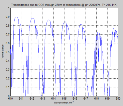
« Newer Posts - Older Posts »