In Part Seven we looked at progressively wider wavelength ranges to see where doubling of CO2 had an impact.
We also compared the top layer of the atmosphere (in that model) with the bottom layer – again seeing very significant differences.
This series is aimed at helping people understand how “greenhouse” gases have the effect that they do.
Now we have a model (described in Part Five) which incorporates the actual line by line absorption and emission of various GHGs in a realistic atmosphere we can play around with “what if” scenarios.
Usually as we go up in altitude and pressure drops, the absorption lines get narrower. Around the tropopause the lines are almost 1/5 of their surface width.
I introduced a new on/off parameter into the code which “turns off” this physics and allows us to keep the lines the same width as at the surface. Then compared 280 to 560 ppm of CO2 under one clear sky condition for the case with and without absorption line narrowing.
The top graph is the difference in TOA spectrum with correct physics. The bottom graph is the same but with all absorption lines at their surface width:
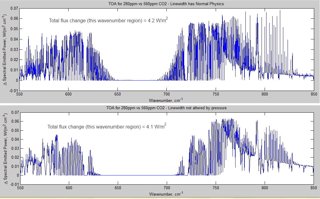
Click to expand
The results surprised me. I expected that the effects of absorption lines narrowing would be more significant for this “increased GHG” scenario.
The difference in outgoing radiation (OLR) across this band (which is most but not all of the CO2 effect) is only 0.1 W/m².
[Update shortly afterwards inspired by comment from Hockey Schtick]
The original article might give the false impression that the narrowing of lines has little effect on TOA flux. Actually it has a significant effect. For example, for the case 280 ppm the difference in total TOA flux for correct – incorrect physics = 23.5 W/m². It’s just that for 560 ppm the difference in total TOA flux for correct – incorrect physics = 24.8 W/m².
The values annotated on the graph are the flux for that wavenumber region only.
TOA flux in the list below is across all wavelengths.
CO2 ppm Line Width TOA flux
280 Narrows with lower pressure 268.4 W/m²
560 Narrows with lower pressure 262.2 W/m²
280 Constant 244.9 W/m²
560 Constant 237.4 W/m²
Difference 280 ppm correct – incorrect physics = 23.5 W/m²
Difference 560 ppm correct – incorrect physics = 24.8 W/m²
Difference 280 ppm – 560 ppm (correct physics) = 6.2 W/m²
Difference 280 ppm – 560 ppm (incorrect physics) = 7.5 W/m²
DLR (downward longwave radiation = atmospheric longwave radiation incident on surface) for the same conditions:
CO2 ppm Line Width DLR flux
280 Narrows with lower pressure 374.7 W/m²
560 Narrows with lower pressure 376.9 W/m²
280 Constant 378.1 W/m²
560 Constant 380.6 W/m²
Difference 280 ppm correct – incorrect physics = -3.4 W/m²
Difference 560 ppm correct – incorrect physics = -3.7 W/m²
Difference 280 ppm – 560 ppm (correct physics) = -2.2 W/m²
Difference 280 ppm – 560 ppm (incorrect physics) = -2.5 W/m²
Related Articles
Part One – some background and basics
Part Two – some early results from a model with absorption and emission from basic physics and the HITRAN database
Part Three – Average Height of Emission – the complex subject of where the TOA radiation originated from, what is the “Average Height of Emission” and other questions
Part Four – Water Vapor – results of surface (downward) radiation and upward radiation at TOA as water vapor is changed
Part Five – The Code – code can be downloaded, includes some notes on each release
Part Six – Technical on Line Shapes – absorption lines get thineer as we move up through the atmosphere..
Part Seven – CO2 increases – changes to TOA in flux and spectrum as CO2 concentration is increased
Part Nine – Reaching Equilibrium – when we start from some arbitrary point, how the climate model brings us back to equilibrium (for that case), and how the energy moves through the system
Part Ten – “Back Radiation” – calculations and expectations for surface radiation as CO2 is increased
Part Eleven – Stratospheric Cooling – why the stratosphere is expected to cool as CO2 increases
Part Twelve – Heating Rates – heating rate (‘C/day) for various levels in the atmosphere – especially useful for comparisons with other models.


Doubled CO2 only “traps” 0.1Wm-2 of OLR ?
Hockey Schtick,
Take a look at the annotation on each of the graphs.
In the case of this 1D clear sky model, the difference in OLR for 280ppm vs 560ppm is 4.2 W/m2. That’s the top graph.
When we use take out a piece of physics from the model and don’t allow the absorption lines to narrow further up in the atmosphere, then the difference in OLR is 4.1 W/m2. That’s the bottom graph.
The difference between correct physics and removing this one piece of physics is a Delta of 0.1 W/m2.
So I ran 4 cases:
280 ppm – correct physics.
560 ppm – correct physics.
280 ppm – no line width changes
560 ppm – no line width changes
Inspired as I usually am by a question or comment from Hockey Schtick I provide further feedback below and will add this material to the article shortly.
The value TOA is the list below is across all wavelengths. The values annotated on the graph are the flux for that wavenumber region only.
280 ppm – correct physics TOA = 268.4 W/m2
560 ppm – correct physics. TOA = 262.2 W/m2
280 ppm – no line width changes. TOA = 244.9 W/m2
560 ppm – no line width changes. TOA = 237.4 W/m2
Difference 280 ppm correct – incorrect physics = 23.5 W/m2
Difference 560 ppm correct – incorrect physics = 24.8 W/m2
Difference 280 ppm – 560 ppm (correct physics) = 6.2 W/m2
Difference 280 ppm – 560 ppm (incorrect physics) = 7.5 W/m2
DLR changes (atmospheric longwave radiation incident on surface):
280 ppm – correct physics DLR = 374.7 W/m2
560 ppm – correct physics. DLR = 376.9 W/m2
280 ppm – no line width changes. DLR = 378.1 W/m2
560 ppm – no line width changes. DLR = 380.6 W/m2
Difference 280 ppm correct – incorrect physics = -3.4 W/m2
Difference 560 ppm correct – incorrect physics = -3.7 W/m2
Difference 280 ppm – 560 ppm (correct physics) = -2.2 W/m2
Difference 280 ppm – 560 ppm (incorrect physics) = -2.5 W/m2
Thanks for the clarification.
Curious what accounts for the difference- you find 4.1Wm-2 at TOA from 2XCO2 vs. IPCC 3.7Wm-2
What does your model claim for forcing at the surface from 2XCO2?
Hockey Schtick:
There is some explanation given about that in the various preceding articles which are all worth having a look through.
In brief, and not complete –
1. This is one clear sky condition for one surface temperature
2. There is no stratospheric adjustment following an increase in CO2 in my model, but that is done in the std definition
3. My stratospheric temperature profile is not correct, it is isothermal whereas the real stratosphere increases with temperature due to solar absorption by various GHGs. The stratospheric radiation balance is important (surprising for such a little amount of atmosphere).
So I would never expect to get the same answer. It would just be chance if that happened.
Hockey Schtick
We will have a look at that in a bit of detail in a forthcoming article.
Please also reveal what your model claims the surface temperature would be for:
1. No IR active gases in the atmosphere, just say 80% nitrogen & 20% oxygen
2. No water vapor or other IR active gases other than CO2,
with CO2 at say 200 ppm, 400 ppm, 800 ppm and 100% of atmosphere
Hockey Schtick
The important thing to understand about the model here, and in the previous articles so far, is that it models the spectrum of up and down radiation through the atmosphere – for a given set of conditions.
That is, if you state the conditions for the temperature profile from the surface up to the tropopause, and the concentrations of all GHGs especially water vapor, the model can tell you the upward spectrum (and flux) at any height, and the downward spectrum (and flux) at any height.
This is the first step to understanding radiative transfer. But also the most important. If we subsequently run to equilibrium we will find that the surface and atmosphere end up at new temperatures.
This model is much less useful for working out an accurate equilibrium temperature because it doesn’t (yet) have atmospheric absorption of solar radiation and doesn’t consider the stratospheric O2 and O3 absorption. And, of course, it is just a 1D radiative-convective model so has other limitations.
The conditions for the above runs were 300K surface temperature, 80% humidity in a boundary layer that reaches 920 hPa, 40% humidity in the atmosphere above (free troposphere), CH4 at 1775 ppbv, N2O at 319 ppbv, no ozone, and CO2 at the concentrations stated. Also the tropopause was set at 200 hPa and the top of model was 50 hPa.
The case of N2 and O2 only is relatively simple. The atmosphere is optically thin as it’s most important interaction with thermal radiation is through the microwave lines of O2. That’s enough to win over conduction. Thus the theory of thin atmosphere presented in the book Pierrehumbert (and certainly also elsewhere) applies.
Assuming that the solar heating can be neglected in the troposphere that leads to a troposphere with dry adiabatic lapse rate up to the level where the temperature is the surface temperature divided by fourth root of 2, i.e. 0.84 times the surface temperature. The atmosphere does not affect significantly the surface temperature which is determined directly by the Stefan-Boltzmann law taking into account the assumed albedo of the surface. As we are discussing a counterfactual case, no model can tell what the albedo is. Thus the resulting (effective average) surface temperature can be anything from extremely low to about 275K, which would be reached, when the albedo for solar SW is 95% of that for thermal IR.
What I would really like to see would be an iterative process towards a doubling of CO2 using small increments say of 28ppm
T=288K
CO2 = 280ppm
loop 100 times
CO2 = CO2+28
calculate change in TOA forcing
calculate DT to balance energy
T = T + DT
endloop
One reason for this is to know if radiative losses through the IR window increase with T or whether CO2 bites more into the window. The analogy pumping air into a tyre with a puncture. The more you pump the more air escapes unless the hole gets smaller.
P.S. I realise this would take a huge amount of CPU time.
Clive,
I’m working towards that at the moment with a model revision.
First of all to see the result for an instantaneous change, and then a gradual change.
The time taken is mostly for the calculation of transmissivity/absorptivity per wavenumber per layer. The subsequent time step energy balance calculations don’t add a lot to it.
Although as an insightful anti-computer friend of mine said to me a long time ago, “they say computers save you time, but no one ever defines t=0“.
And this is how I find it. The time taken is getting the updated code to work and verifying it.
I’m updating the code with time steps and adding the tracking of total energy movement for surface & all atmospheric layers along with a subset of convective energy for all layers.
I have looked through and understand the code plus ordered a copy of HITRAN. The problem will be buying MATLAB so I may adapt it to something else.
What has surprised me most is that the main CO2 “greenhouse” effect is concentrated in the lines at the side of the central line. This is because they are not saturated below the tropopause.
If you look at a typical spectrum from space for example this one , then you see the an upward peak at the central 15 micro line. Why is this ? Is it this because the emission height is so high in the stratosphere that the temperature is now higher than the tropopause ?
Clive,
Your proposal is correct. The sharp peak at the center of the CO2 line originates in the upper stratosphere where the temperature is higher due to heating by solar UV. The peak is very narrow, because it originates from altitudes where the pressure is very low. Doppler broadening may be the main determinant of the line shape for that peak.
Clive,
Spot on.
You can see some similar curves – reproduced from Grant Petty’s excellent book – along with explanation in Understanding Atmospheric Radiation and the “Greenhouse” Effect – Part Ten.
If you don’t get the opportunity to get a copy of the amazing Matlab then there is always the pathway of requesting to see the Matlab model simulating the climate in a certain way.
Definitely no promises, but half of what I anyway produce in articles is based on either questions, claims, comments, or my perception of the issues in the blogosphere.
Clive,
To study, how changes occur, a radiative transfer model is not enough but it must be complemented by a dynamic atmospheric model that can calculate changes in convection and in the energy content of various subsystems even for the no-feedback case. For more realism it must be possible to include the feedbacks as well.
A minimum alternative would be an one-dimensional atmospheric model which could perhaps used in a way that allows handling both the rising and the subsiding convection.
Perhaps SoD is considering such additions to his toolset (I have no knowledge on that). It would be a significant extra effort, but perhaps still feasible.
I wrote my comment before I saw SoD’s above comment.
Pekka,
Your comment is correct, but I am not creating a GCM.
I believe there is still a lot of value in demonstrating how the energy moves around in a 1D radiative-convective model after a GHG concentration is changed, or while a GHG concentration is changed.
Most of the reactions against how the greenhouse effect works, or responds to changes in GHG concentration, are because of the conceptual models that most people carry. They trust their conceptual models over the physics.
We will see.
What I had in mind is something like the single shell model of Pierrehumbert (1995) that you discussed recently, but probably with significant modifications in the details.
It would have one flow up, one down and perhaps a way of mixing the flows.
Such a model could be coupled to the radiation model.
“Your proposal is correct. The sharp peak at the center of the CO2 line originates in the upper stratosphere”
Disagree. The Planck temperatures are way too low. Furthermore, all CO2 radiance observed by Nimbus is in the lower stratosphere in a remarkably narrow range.
gymnosperm,
So it’s lower stratosphere. The important point is that it originates above the tropopause where temperature is increasing. And you see some structure because the pressure is low.
Somewhat off topic, but not entirely: Does CO2 introduced into the high troposhere or stratosphere, say by a passing jet, result in the same distribution of CO2 through the entire atmosphere, as that introduced on the ground, say by a car’s tailpipe? I suspect yes, reaches same equilibrium eventually, but does it take minutes, hours, days, months?
If you look at annual averages, comparing the South Pole CO2 data with the data from Barrow, AK, there’s about a two year lag. I would think it would take even longer to cross the tropopause. Chlorine in the stratosphere in the mid-latitudes didn’t start to decline until 1997, ten years after the ratification of the Montreal Protocol.
scienceofdoom on January 15, 2013 at 1:21 am
My stratospheric temperature profile is not correct, it is isothermal whereas the real stratosphere increases with temperature due to solar absorption by various GHGs.
Even without solar heating, the temperature increases with decreasing altitude. With this increase in temperature also increases the temperature gradient and thereby ultimately sets the convection on = tropopause: the transition from the stratosphere into the troposphere.
Even without solar heating, the temperature increases with decreasing altitude. With this increase in temperature also increases the temperature gradient and thereby ultimately is beginning the convection = tropopause: the transition from the stratosphere into the troposphere.
Pekka Pirilä on January 17, 2013 at 9:18 am
“The case of N2 and O2 only is relatively simple. The atmosphere is optically thin as it’s most important interaction with thermal radiation is through the microwave lines of O2. That’s enough to win over conduction.
…
Assuming that the solar heating can be neglected in the troposphere that leads to a troposphere with dry adiabatic lapse rate up to the level where the temperature is the surface temperature divided by fourth root of 2, i.e. 0.84 times the surface temperature.”
No dry adiabatic lapse rate. The largest part of the atmosphere is uniform warm – as the warmest location of the earth’s surface. The warm atmosphere is separated from the surface mostly cooler by an inversion layer. The inversion layer is still air and still air is a poor conductor of heat.
Ebel,
Wrong. The atmosphere is a poor conductor of heat, but it still conducts. The conduction path to the surface is measured in tens of kilometers, the path to the equator is in thousands of kilometers. There is no way that conduction from the equator is going to predominate in an atmosphere with no circulation. If you allow any circulation at all, you must get a near adiabatic lapse rate with the potential temperature, not the actual temperature, approximately equal to the warmest point on the surface. And you have neglected heat loss by radiation from the oxygen microwave lines. That will be more effective than conduction too.
Oh, and there will also be significant radiative heat loss from collision induced absorption/emission as well. I’m betting that will be even higher than the microwave emission from oxygen as it’s at shorter wavelength, ~100μm peak.
Ebel,
Your description is what I have proposed for the case where absolutely no radiative heat transfer occurs. DeWitt has argued against this proposal, but I continue to consider it quite plausible. What would happen in that case depends on the roles conduction has in two very weak processes. I.e. the approach towards isothermal on the one hand and conduction trough the inversion layer to areas with colder surface on the other. I consider this question unresolved but personally still prefer the mostly isothermal alternative.
The case discussed here is, however, different as long as we have O2 in the atmosphere, because O2 has bands in microwave frequencies and microwaves do also transfer energy similarly with IR. The microwaves are only much less effective in that. Because conduction is an extremely weak form of energy transfer in the atmosphere, the microwave based transfer is likely to dominate by orders of magnitude. That would be just a perfect case of the optically thin atmosphere. That’s why I mentioned microwaves already in my earlier message. Microwaves lead also to weak emission from all levels of atmosphere to the space cooling weakly the upper atmosphere.
The weak cooling of the upper atmosphere would be enough to support weak convection up to the tropopause at an altitude of around 4 km. If the absorption of solar SW is significant still at this altitude the troposphere would get thinner as warming by SW enters the formula that determines the temperature of the tropopause of an optically thin atmosphere. In absence of this effect the tropopause would be about 40 C colder than the surface.
There are additional complications from the large spatial and temporal variability of the surface temperature. That would certainly influence the atmospheric circulation but I don’t dare to speculate more on that.
Pekka,
Thought experiment: Consider an atmosphere with zero thermal conductivity. That will only be isothermal if it starts out isothermal. Otherwise you get the entire atmosphere with constant potential temperature because there’s no mechanism for heat conduction to make the atmosphere isothermal, even in the 1D case, once convection stops. IMO, you only get an isothermal atmosphere in the limiting case of infinite conductivity where the surface will be isothermal too. As long as the surface isn’t isothermal, there must be some convection/advection in the bulk of the atmosphere, not just the surface layer. Once again, horizontal paths are at least two orders of magnitude larger than vertical paths and the temperature gradient is smaller too. That cannot make the atmosphere isothermal. Only if you allow horizontal conductivity to be orders of magnitude higher than vertical conductivity could you possibly get something like the atmosphere you propose.
If we make the atmosphere infinitely viscous, the temperature at the pole at 500hPa, or about 5.5 km altitude, must be such that heat loss to the ground equals heat gain from the equator, 10,000km distant. The pole is going to be greater than 200K colder than the equator, assuming that the axis of rotation is perpendicular to the orbital plane. How can you possibly imagine an isothermal atmosphere?
DeWitt,
How my intuition tells that the state of the atmosphere develops with exactly zero emissivity.
The surface will reach the maximum temperature at one point that moves as Earth rotates. The atmosphere is always at least a little cooler than that point. Some convection results. That brings heat to the upper atmosphere. There’s always at least some dissipation. Dissipation adds a little to the temperature of air. That leads to the situation that air in the upper troposphere exceeds soon the value given by adiabat, i.e. some stratification is created. Due to this stratification the rising air cannot rise as high anymore.
As the atmosphere is heated from the hottest spot, an inversion develops everywhere. Thus we have a strong heating mechanism for the atmosphere but only conduction as a mechanism for cooling. Heat continues to be added to the atmosphere until the temperature of the atmosphere is very close to that of the hottest spot.
The top of the convective atmosphere moves gradually lower and lower. That continues until the very little circulation left is squeezed in a thin layer just above the layer of inversion. That thin layer of circulation is cooled by conduction through the thin layer of inversion and warmed at the hottest spot. In the stationary state the conduction through the inversion is the limiting factor that determines the total power involved in the circulation. The temperature of the circulating layer settles at a value that makes the convective heating at the hot spot equal to the conductive cooling elsewhere.
The weak circulation is close to laminar but some turbulence is always present. That leads to a little turbulent mixing that adds to the conduction a little, but very little in a strongly stratified atmosphere. The inversion layer as a very strong stratification and is thus stable. The upper atmosphere has been effectively isolated from the circulation and even the very weak conduction is enough to strengthen the stratification and ultimately makes all that isothermal.
What’s left is
– A thin layer of strong inversion at the bottom (except at the hot spot)
– A thin layer of circulation on top of that
– A warm isothermal atmosphere in all the rest of the atmosphere
The power involved in the circulation is very low and determined by conduction through the layer of inversion
That’s how I see it.
Pekka,
I think you’re still ignoring the vast differences in area and distance involved. You only get heating from a very small area near the equator. You get cooling everywhere else.
The strong heating mechanism goes away as soon as the atmosphere stratifies, which it does when the potential temperature stops decreasing with altitude. Now there is no strong heating mechanism for the rest of the atmosphere. Effectively all the incoming energy is radiated away locally. For a 1D atmosphere, conduction will eventually lead to an isothermal atmosphere.
But the atmosphere isn’t one dimensional. There is a large temperature gradient from the equator to the poles. Any temperature inversion means the atmosphere there is on average cooler than at the equator. That means there will be a pressure gradient that increases with altitude.
Now you can increase the thickness of the inversion layer to make conduction arbitrarily small, but it’s still going to be greater than that for what you claim to be a nearly isothermal atmosphere over a distance of more than three orders of magnitude larger. And, it only increases the pressure gradient force. You have to invoke a highly turbulent atmosphere above the inversion layer to make it isothermal, there is no mechanism to generate that turbulence once the lapse rate reaches the adiabatic rate. There is only conduction. But conduction cuts both ways.
No, it hasn’t. Any flow towards the equator just above the inversion layer will be balanced by flow in the opposite direction at higher altitude. You’ll still have pressure gradient force because the inversion layer, which gets thicker with increasing latitude, will still cause the pressure to decrease more rapidly with altitude than at the equator. You can’t have flow in both directions in a thin layer. That colder air will be warmed at the equator and rise. Even a tiny flow upward will be enough to keep a near adiabatic lapse rate at the equator. If the lapse rate is adiabatic at the equator, it can’t be zero in the rest of the atmosphere.
Your model implies a discontinuity at zero absorptivity as the atmosphere becomes more transparent. I don’t think that’s good physics. Of course it’s all moot, because there’s no such thing as a perfectly transparent atmosphere.
DeWitt,
One of your points is easy to answer. There isn’t any relevant discontinuity at zero conductivity.
First of all zero conductivity is not part of a continuum and it’s role is more easily understandable in terms of thermal resistivity: zero conductance is infinite resistivity. Reaching the equilibrium takes a very long time that grows at least linearly in resistivity. In the limit of infinite resistivity it will never be reached.
The rest is more complex. The inversion layer near surface would be very thin near the hot spot and it would have a maximum thickness near poles. The top level of the convective layer would have its maximum altitude at the hot spot and essentially meat the top of inversion at the poles. The potential temperature would increase with altitude everywhere except at the hot spot where it would decrease slightly from surface to the top of the uplift. Estimating this maximum altitude involved in the stationary convection would take some effort. I have only my intuition to tell that it’s much less than the present altitude of the tropopause or that obtained in the case of optically thin atmosphere where radiative heat transfer still dominates. It might be a few hundred meters, but that’s just a guess.
One thing that I have ignored but that I might actually be important is the influence of mountains and high plateaus. They might have enough influence to push the top of the convective layer much higher. Thus my ideas were really thought to apply only to an Earth with no surface contour.
Pekka,
I think you may be conflating vertical stability with horizontal stability. You get a temperature inversion when the air is calm, not the other way around. There is no reason I can see that a thick inversion layer would be stable in the presence of horizontal air movement, which must be present.
DeWitt,
I haven’t tried to write the equations that control the situation. It seems, however, plausible in my view that the way the circulation is driven by the uplift at the hotspot and the way cooling contributes at each latitude to the return flow would maintain the horizontal pressure gradient needed for the stability of the configuration.
Pekka,
Try reading Chapter 6 of Caballero’s PhysMet lecture notes starting on page 142 of the pdf. My math is severely rusty, but the way I read it is if the potential temperature gradient is positive, you get eddy diffusion of heat down the gradient, i.e. towards the surface, not up. Heat flow in either direction only stops at neutral stability. That says to me that an isothermal atmosphere above a non-isothermal surface isn’t stable. But an atmosphere with constant potential temperature with altitude is stable.
The idea that you could ever get laminar flow over the lengths and temperature gradients involved with a sphere illuminated from a point source doesn’t seem right either.
DeWitt,
There are certainly many points where the solution that I have proposed may fail, but I wouldn’t trust many conclusions based on theories of the real atmosphere in estimating what would happen with exactly zero emissivity. The fundamental equations remain true, but the conditions are so different from those people are used to consider that the solutions may be very different.
You may have noticed that I have given some thought to most of the issues that you have brought up, but I haven’t really done any calculations. It may well be that the relevant Reynolds number turns out to be so high that turbulence is essential, but that again should be calculated, when it’s first understood, what is the right way of defining it for this problem.
A stratified atmosphere is basically stable as shown by stratosphere. One way of describing my proposal is just saying that the altitude of the tropopause would be much lower than presently and also much lower than for an optically thin atmosphere. Adding conduction to the formula of the tropopause temperature of an optically thin atmosphere brings it closer to the surface. In some sense my idea is just an extension of that.
Pekka,
I think you’re completely wrong about this. The existence of the stratosphere and its stability depend entirely on the ability of oxygen to absorb UV radiation and form a significant concentration of ozone at low pressure, which absorbs even more UV radiation. This results in an anti-greenhouse effect because the SW absorptivity is higher than the LW absorptivity. That’s what causes the tropopause. In the absence of oxygen, there would be no stratosphere or mesosphere, just a direct transition to the thermosphere at very high altitude. The Martian atmosphere, for example, doesn’t have a stratosphere.
If I’m so mistaken on the stratosphere, I’m in good company with people like Pierrehumbert whose book on planetary atmospheres has been the most important source for me in learning about the nature of the stratosphere and factors that determine the altitude of the tropopause.
DeWitt,
Do you mean the existence of a stratosphere that increases in temperature? Or the existence of a stratosphere as defined by convection stopping?
I’m in agreement with Pekka that a stratosphere occurs in the absence of solar heating of the upper atmosphere. The atmosphere is so optically thin that the lapse rate would be less than the adiabatic lapse rate and so convection ceases.
SoD,
Convection doesn’t stop when the lapse rate is less than the adiabatic rate.
That takes an inversion layer. Look at typical atmospheric soundings, specifically Figure 2.14 in Caballero. There is a nearly steady increase in the potential temperature from the surface upward.
Fly into Los Angeles on a smoggy day. The location of the inversion layer is obvious.
If an optically thin atmosphere must be stratified, then why is there no stratosphere in the Martian atmosphere? See for example: THE MARTIAN UPPER ATMOSPHERE
DeWitt,
You should check better, what textbooks tell. In the cases that textbooks consider and that simple models can describe the convection stops as soon as the actual lapse rate is less than the adiabatic one for the local composition of air.
In real atmosphere we have all kind of weather phenomena etc. that make things more complex, but the same principles apply even then.
What happens in my model calculations is that the lapse rate produced by radiative effects alone drops below the externally specified lapse of 6.5 K/km rate at about 13 km altitude. Beyond that altitude the lapse rate drops almost immediately to a rather small value.
In the case of an optically thin atmosphere, there are two discrete alternatives. Up to the tropopause convection brings extra heat to supply energy that is radiated half down and half up. As the atmosphere is optically thin the only other significant source of heat is radiation directly from the surface. Radiation from atmosphere is so much weaker in that limit that it can be dismissed as source of energy. At tropopause and above the temperature of the atmosphere is so much lower than at the surface that it radiates at the same power that it absorbs radiation from the surface.
As atmosphere radiates both up and down but surface is only below, that leads to the temperature of the surface temperature divided by the fourth root of 2. That balance is true at all higher altitudes, but in troposphere we have also convection.
In the real atmosphere and in the model of SoD, the radiation from other parts of atmosphere must be taken into account and that results in what you can see in our calculations including those linked to in my recent comment.
Whether the Martian atmosphere has an stratosphere or not is in part a semantic question as far as I can see. It’s different from the Earth atmosphere but what’s called mesosphere in that paper has many properties of a stratosphere and might perhaps also be referred to as stratosphere.
There’s also another important factor and that’s that the Martian atmosphere is not optically thin at the frequencies of the CO2 peaks, which are also very narrow due to the combination of very low pressure and low temperature. That’s probably the reason for the high altitude of the Martian tropopause.
Pekka,
I probably haven’t been precise enough. I should have been talking about circulation rather than convection. But that ‘s the problem when dealing with results from a one-dimensional model.
Without an inversion layer, there is no barrier to circulation. That’s the problem with your definition of the tropopause as being where both convective energy transfer stops for a one-dimensional radiative/convective model and for circulation to stop. As long as there is a latitudinal temperature gradient at the surface, circulation cannot entirely cease. And it won’t be limited to a thin layer just above the surface boundary layer either.
Another problem is the arbitrary choice of a constant stable lapse rate. As the specific humidity declines, the stable lapse rate should approach the dry adiabatic rate rather than some arbitrary value quite a bit less than that. That, as I wrote elsewhere, is the source of the break point in your calculated lapse rate profile.
DeWitt,
From the point of view of convection and circulation the dividing line is the adiabatic lapse rate. There’s nothing special to separate inversion from temperature falling weakly with altitude.
It’s certainly true that a large deviation from the adiabatic lapse rate has a stronger influence than a small deviation. An inversion is an example of large deviations, but that’s all for this question.
To see, how vertical convection can proceed we must consider potential temperature, not temperature.
For those who are reading this and don’t have any appropriate text books I propose the Chapter 2.21 of Caballero’s lecture notes on static stability.
The lecture notes can be found by Googling “PhysMetLectNotes Caballero”. The 2012 version from Sweden is probably most recent.
If you’re too lazy to use a search engine, here’s the link:
Click to access PhysMetLectNotes.pdf
clivebest on January 15, 2013 at 10:13 am
„This is because they are not saturated below the tropopause.“
There is no saturation. Where is strongly absorbed is emitted strong.
“… then you see the an upward peak at the central 15 micro line. Why is this ? Is it this because the emission height is so high in the stratosphere that the temperature is now higher than the tropopause?”
The intensity of a line is dependent on the average temperature along the absorption length. In the middle (15 µm) of the absorption length is so short, that it only goes down into the warm ozone layer.
[…] In fact, the differences are small except in the mid-stratosphere and we may find that this is due to slight differences in the model atmosphere used, or as a result of not using the Voigt profile (this is an important but technical area of atmospheric radiation – line shapes and how they change with pressure and temperature in the atmosphere – see for example Part Eight – CO2 Under Pressure). […]
[…] Visualizing Atmospheric Radiation – Part Six – Technical on Line Shapes Visualizing Atmospheric Radiation – Part Eight – CO2 Under Pressure […]
[…] Part Eight – CO2 Under Pressure – how the line width reduces (as we go up through the atmosphere) and what impact that has on CO2 increases […]
[…] Part Eight – CO2 Under Pressure – how the line width reduces (as we go up through the atmosphere) and what impact that has on CO2 increases […]
[…] Part Eight – CO2 Under Pressure – how the line width reduces (as we go up through the atmosphere) and what impact that has on CO2 increases […]
[…] Part Eight – CO2 Under Pressure – how the line width reduces (as we go up through the atmosphere) and what impact that has on CO2 increases […]
[…] Part Eight – CO2 Under Pressure – how the line width reduces (as we go up through the atmosphere) and what impact that has on CO2 increases […]
In a historical vein, the paper:
P. E. Martin, E. F. Barker, “The infrared absorption spectrum of carbon dioxide”, PHYSICAL REVIEW, 41, 1st August 1932, 291-303.
is one of the earliest I’ve found which has great detail regarding CO2 aborbtion lines.