In Latent heat and Parameterization I showed a formula for calculating latent heat transfer from the surface into the atmosphere, as well as the “real” formula. The parameterized version has horizontal wind speed x humidity difference (between the surface and some reference height in the atmosphere, typically 10m) x “a coefficient”.
One commenter asked:
Why do we expect that vertical transport of water vapor to vary linearly with horizontal wind speed? Is this standard turbulent mixing?
The simple answer is “almost yes”. But as someone famously said, make it simple, but not too simple.
Charting a course between too simple and too hard is a challenge with this subject. By contrast, radiative physics is a cakewalk. I’ll begin with some preamble and eventually get to the destination.
There’s a set of equations describing motion of fluids and what they do is conserve momentum in 3 directions (x,y,z) – these are the Navier-Stokes equations, and they conserve mass. Then there are also equations to conserve humidity and heat. There is an exact solution to the equations but there is a bit of a problem in practice. The Navier-Stokes equations in a rotating frame can be seen in The Coriolis Effect and Geostrophic Motion under “Some Maths”.
Simple linear equations with simple boundary conditions can be re-arranged and you get a nice formula for the answer. Then you can plot this against that and everyone can see how the relationships change with different material properties or boundary conditions. In real life equations are not linear and the boundary conditions are not simple. So there is no “analytical solution”, where we want to know say the velocity of the fluid in the east-west direction as a function of time and get a nice equation for the answer. Instead we have to use numerical methods.
Let’s take a simple problem – if you want to know heat flow through an odd-shaped metal plate that is heated in one corner and cooled by steady air flow on the rest of its surface you can use these numerical methods and usually get a very accurate answer.
Turbulence is a lot more difficult due to the range of scales involved. Here’s a nice image of turbulence:
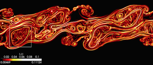
From NASA – http://www.nas.nasa.gov/SC12/demos/demo28.html
Figure 1
There is a cascade of energy from the largest scales down to the point where viscosity “eats up” the kinetic energy. In the atmosphere this is the sub 1mm scale. So if you want to accurately numerically model atmospheric motion across a 100km scale you need a grid size probably 100,000,000 x 100,000,000 x 10,000,000 and solving sub-second for a few days. Well, that’s a lot of calculation. I’m not sure where turbulence modeling via “direct numerical simulation” has got to but I’m pretty sure that is still too hard and in a decade it will still be a long way off. The computing power isn’t there.
Anyway, for atmospheric modeling you don’t really want to know the velocity in the x,y,z direction (usually annotated as u,v,w) at trillions of points every second. Who is going to dig through that data? What you want is a statistical description of the key features.
So if we take the Navier-Stokes equation and average, what do we get? We get a problem.
For the mathematically inclined the following is obvious, but of course many readers aren’t, so here’s a simple example:
Let’s take 3 numbers: 1, 10, 100: the average = (1+10+100)/3 = 37.
Now let’s look at the square of those numbers: 1, 100, 10000: the average of the square of those numbers = (1+100+10000)/3 = 3367.
But if we take the average of our original numbers and square it, we get 37² = 1369. It’s strange but the average squared is not the same as the average of the squared numbers. That’s non-linearity for you.
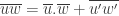
In the Navier Stokes equations we have values like east velocity x upwards velocity, written as uw. The average of uw, written as 

When we create the Reynolds averaged Navier-Stokes (RANS) equations we get lots of new terms like
It’s like saying x + y = 1, what is x and y? No one can say. Perhaps 1 & 0. Perhaps 1000 & -999.
Digression on RANS for Slightly Interested People
The Reynolds approach is to take a value like u,v,w (velocity in 3 directions) and decompose into a mean and a “rapidly varying” turbulent component.
So 


And
So in the original equation where we have a term like 

So 2 unknowns instead of 1. The first term is the averaged flow, the second term is the turbulent flow. (Well, it’s an advection term for the change in velocity following the flow)
When we look at the conservation of energy equation we end up with terms for the movement of heat upwards due to average flow (almost zero) and terms for the movement of heat upwards due to turbulent flow (often significant). That is, a term like 
Or, in plainer English, how heat gets moved up by turbulence.
..End of Digression
Closure and the Invention of New Ideas
“Closure” is a maths term. To “close the equations” when we have more unknowns that equations means we have to invent a new idea. Some geniuses like Reynolds, Prandtl and Kolmogoroff did come up with some smart new ideas.
Often the smart ideas are around “dimensionless terms” or “scaling terms”. The first time you encounter these ideas they seem odd or just plain crazy. But like everything, over time strange ideas start to seem normal.
The Reynolds number is probably the simplest to get used to. The Reynolds number seeks to relate fluid flows to other similar fluid flows. You can have fluid flow through a massive pipe that is identical in the way turbulence forms to that in a tiny pipe – so long as the viscosity and density change accordingly.
The Reynolds number, Re = density x length scale x mean velocity of the fluid / viscosity
And regardless of the actual physical size of the system and the actual velocity, turbulence forms for flow over a flat plate when the Reynolds number is about 500,000. By the way, for the atmosphere and ocean this is true most of the time.
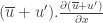
Kolmogoroff came up with an idea in 1941 about the turbulent energy cascade using dimensional analysis and came to the conclusion that the energy of eddies increases with their size to the power 2/3 (in the “inertial subrange”). This is usually written vs frequency where it becomes a -5/3 power. Here’s a relatively recent experimental verification of this power law.
From Durbin & Reif 2010
Figure 2
In less genius like manner, people measure stuff and use these measured values to “close the equations” for “similar” circumstances. Unfortunately, the measurements are only valid in a small range around the experiments and with turbulence it is hard to predict where the cutoff is.
A nice simple example, to which I hope to return because it is critical in modeling climate, is vertical eddy diffusivity in the ocean. By way of introduction to this, let’s look at heat transfer by conduction.
If only all heat transfer was as simple as conduction. That’s why it’s always first on the list in heat transfer courses..
If have a plate of thickness d, and we hold one side at temperature T1 and the other side at temperature T2, the heat conduction per unit area:

where k is a material property called conductivity. We can measure this property and it’s always the same. It might vary with temperature but otherwise if you take a plate of the same material and have widely different temperature differences, widely different thicknesses – the heat conduction always follows the same equation.
Now using these ideas, we can take the actual equation for vertical heat flux via turbulence:

where w = vertical velocity, θ = potential temperature
And relate that to the heat conduction equation and come up with (aka ‘invent’):

Now we have an equation we can actually use because we can measure how potential temperature changes with depth. The equation has a new “constant”, K. But this one is not really a constant, it’s not really a material property – it’s a property of the turbulent fluid in question. Many people have measured the “implied eddy diffusivity” and come up with a range of values which tells us how heat gets transferred down into the depths of the ocean.
Well, maybe it does. Maybe it doesn’t tell us very much that is useful. Let’s come back to that topic and that “constant” another day.
The Main Dish – Vertical Heat Transfer via Horizontal Wind
Back to the original question. If you imagine a sheet of paper as big as your desk then that pretty much gives you an idea of the height of the troposphere (lower atmosphere where convection is prominent).
It’s as thin as a sheet of desk size paper in comparison to the dimensions of the earth. So any large scale motion is horizontal, not vertical. Mean vertical velocities – which doesn’t include turbulence via strong localized convection – are very low. Mean horizontal velocities can be the order of 5 -10 m/s near the surface of the earth. Mean vertical velocities are the order of cm/s.
Let’s look at flow over the surface under “neutral conditions”. This means that there is little buoyancy production due to strong surface heating. In this case the energy for turbulence close to the surface comes from the kinetic energy of the mean wind flow – which is horizontal.
There is a surface drag which gets transmitted up through the boundary layer until there is “free flow” at some height. By using dimensional analysis, we can figure out what this velocity profile looks like in the absence of strong convection. It’s logarithmic:
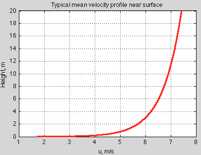
Figure 3 – for typical ocean surface
Lots of measurements confirm this logarithmic profile.
We can then calculate the surface drag – or how momentum is transferred from the atmosphere to the ocean – using the simple formula derived and we come up with a simple expression:

Where Ur is the velocity at some reference height (usually 10m), and CD is a constant calculated from the ratio of the reference height to the roughness height and the von Karman constant.
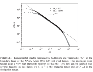
Using similar arguments we can come up with heat transfer from the surface. The principles are very similar. What we are actually modeling in the surface drag case is the turbulent vertical flux of horizontal momentum 
Adding the Richardson number for non-neutral conditions we end up with a temperature difference along with a reference velocity to model the turbulent vertical flux of sensible heat 

Now with a bit more maths..
At the surface the horizontal velocity must be zero. The vertical flux of horizontal momentum creates a drag on the boundary layer wind. The vertical gradient of the mean wind, U, can only depend on height z, density ρ and surface drag.
So the “characteristic wind speed” for dimensional analysis is called the friction velocity, u*, and

This strange number has the units of velocity: m/s – ask if you want this explained.
So dimensional analysis suggests that 
So a simple re-arrangement and integration gives:

where z0 is a constant from the integration, which is roughness height – a physical property of the surface where the mean wind reaches zero.
The “real form” of the friction velocity is:

we can pick a horizontal direction along the line of the mean wind (rotate coordinates) and come up with:

If we consider a simple constant gradient argument:

where the first expression is the “real” equation and the second is the “invented” equation, or “our attempt to close the equation” from dimensional analysis.
Of course, this is showing how momentum is transferred, but the approach is pretty similar, just slightly more involved, for sensible and latent heat.
Conclusion
Turbulence is a hard problem. The atmosphere and ocean are turbulent so calculating anything is difficult. Until a new paradigm in computing comes along, the real equations can’t be numerically solved from the small scales needed where viscous dissipation damps out the kinetic energy of the turbulence up to the large scale of the whole earth, or even of a synoptic scale event. However, numerical analysis has been used a lot to test out ideas that are hard to test in laboratory experiments. And can give a lot of insight into parts of the problems.
In the meantime, experiments, dimensional analysis and intuition have provided a lot of very useful tools for modeling real climate problems.


The scaling of wind shear in the boundary layer is apparently from Monin and Obukhov, 1954.
There is an element of mixing in the atmosphere that I don’t think you are taking into account and that involves the jet stream and a plasma phase of water that allows/enables the jet stream to be isolated from friction that would normally be associated with a larger flow, and which allows/enables it to be the source of high speed windshear in the atmosphere. For more on this:
Regards,
SoD,
Very nice explanation.
Viscous dissipation of energy takes place under any shear rate regime, not just turbulent. I am sure you know this, but your post might give some the impression that it only is present when flow is turbulent.
It might be informative to compare the magnitude of vertical transport of heat due to turbulent flow with uniform potential temperature (as you did here) with vertical transport of heat under different atmospheric ‘stability’ conditions. Seems to me that the rate of vertical transport from the surface has to be very sensitive to the profile of potential temperature, with huge increases when the atmosphere is ‘warmer’ below and ‘cooler’ above (in potential rather than sensible temperature), and large decreases when it is the other way around (that is, when there is a thermal inversion in a potential temperature sense).
I think this is relevant to GCM’s because we live in the surface boundary layer, and boundary layer vertical transport seems to me an important factor in determining how surface temperatures are going to change with increases in GHG forcing.
Testing using Pekka’s latex tips..
overbars are much easier to read (I think) than the brackets in longer expressions..
2nd to last equation:
the last equation:
An earlier equation:
So Latex works great in the comments. See Pekka’s tips for how to.
I tried inserting this into the article itself but it just shows up as the text. I inserted in the “text” field of WordPress rather than the usual WYSIWYG editor. The “text” field is where I have to type in all the cumbersome html to code up superscripts and subscripts.
I’m sure that if this hosted WordPress supports Latex equations in the comments, there must be a way to get these in the article..
Any suggestions?
Scratch that last question. You type the equation into the WYSIWYG editor and it shows up as text, but in preview it shows up as the equation.
And updated the article with hopefully easier to read equations.
I noticed the comment in the text:”Why do we expect that vertical transport of water vapor to vary linearly with horizontal wind speed? Is this standard turbulent mixing?”
My answer would be that ON AVERAGE there is little effect on vertical transport of water vapor from any process on Earth. There certainly could be local effects, but they have to be compensated for globally. Consider: all evaporated water has to eventually condense and rain or snow out, to be replaced by new water vapor. The amount of evapotranspiration on average removes about 86.4 W/m2 from the surface, and about 40.1 W/m2 radiates directly to space from the surface (both on average). Since the only NET energy absorbed on the surface is 163.3 W/m2 of solar radiation (subsurface heating is less than 0.09 W/m2), the only remaining net energy removal is thermals (conduction/convection) of about 18.4 W/m2, and NET radiation from the surface to the atmosphere (398.2 W/m2 up – 340.3 W/m2 down) of 18.4 W/m2. It is clear that average direct radiation to space is not going to change with wind or mixing. The average net radiation to atmosphere also will not change much with wind or mixing. The only significant change would be thermal heat transfer, which would increase with wind and turbulence, which thus would tend to DECREASE evapotranspiration. Since the average total atmospheric water content is balanced, trying to force more water up just sucks up the energy lost by thermals, and the same forces that do this also push up thermal heat transfer. The two processes are competing for the same average solar energy. You can’t do this on average, only locally for a limited time by drawing on stored energy (from deeper in the ground or water). Only 163.3 W/m2 is available to be removed on average! Thus there is no way to change the average evaporation at the surface.
Leonard,
I think you are holding the wrong things constant in your argument.
Radiation is a function of temperature. So if you move heat out of the surface via sensible/latent heat due to increased winds then the radiation from the surface to the atmosphere will reduce. If you move more heat into the atmosphere the radiation from the atmosphere to the surface will increase. So the net radiation will change.
To take an extreme case, if all the surface winds went to zero then the balance of energy will change.
You would have less moisture in the atmosphere for one.
You could try a different tack and argue that local convection due to instability totally overwhelms any convection caused by turbulent mixing from surface winds. That would be a completely different argument.
It seems that your current argument is based on using current averages which come from current climate conditions and somehow these cannot change.
Maybe I misunderstand what you are putting forward.
Flux of sensible heat is proportional to the vertical gradient of potential temperature and that of latent heat to the vertical gradient of absolute humidity. Both depend on the strength of mixing and thus on winds.
The net IR flux is approximately linearly dependent on the temperature gradient, but the coefficient of that dependency is not very high (far less than what would make it proportional). The net IR flux depends also strongly on cloudiness and on absolute humidity.
The fluxes at different altitude must satisfy conservation of energy and mass taking into account condensation that contributes both the sensible heat balance and mass balance of water.
Combining all the above in a quantitative manner tells on the average shares of various components of energy transfer. It should be possible to understand roughly the relative importance of latent heat transfer using as input only a few facts on the atmospheric profile. I haven’t checked, how far that approach can bring us.
The lapse rate is essentially constant (it would decrease slightly with increased evapotranspiration, but this term is already very large and can’t get much larger). As long as there is sufficient mixing to maintain it, more mixing would not change this. Since radiation to space and evapotranspiration greatly dominate net heat transfer up, changing the much smaller thermals and radiation terms a modest portion of their level would have a very small net effect. Since the thermals and radiation to atmosphere are both driven in the same direction by increased mixing, I do not expect a significant trade off or net change between these effects with more wind or turbulence. There are extreme possible cases where this could change, but they require there not be enough mixing to maintain the basic physical processes, and are not relevant for the real Earth. Very strong wind and turbulence would change the very near surface properties (lower few m), but I am referring to the overall atmosphere.
It is also true that at higher overall temperatures, due to increased absorbing gases, that net radiation transfer to the atmosphere would decrease (slightly at realistic temperatures), even though both radiation up and back radiation increase. Thermals would likely increase to compensate. Radiation to space would likely change little (less radiation window, but greater temperature radiation compensating). Evapotranspiration might change a small amount, but not much.
Leonard,
I thought it would be easier to prove you wrong and demonstrate that turbulent mixing has a big effect.
Perhaps I’ve now confused myself. Or maybe I was confused all along..
I started writing a description and realized it had flaws.
Basically, turbulent mixing for nighttime conditions and daytime conditions (in tropical/sub-tropical cloudless locations) works in opposite directions. At least as far as transferring heat between the surface and the boundary layer of the atmosphere.
I’m not thinking about the condition where solar insolation warms the surface sufficiently to initiate convection. I’m thinking about how that convection condition is delayed in the morning for zero winds vs winds – and how that condition is ended earlier with winds vs zero winds. Seems like there are two opposite effects.
But the boundary layer atmosphere isn’t a fixed condition either.
I’m about to head off for a lot of travel. I will try and think about this more in the coming days.
Leonard and SOD: If all other factors are kept unchanged, convective cooling increases at the same rate as the saturation vapor pressure – 7%/K or 6 W/m2/K using Leonard’s value for latent heat.
LE = ρ_a*L*CE*U*q_w*(1 − RH)
If Leonard were right, 2.5 degC of surface warming theoretically should reduce the flux of simple heat to zero, which isn’t likely. However, Leonard correctly notes that unless the extra water vapor can escape the boundary layer and condense, evaporative cooling will be shut down by rising RH in the boundary layer. In the tropics, deep convection may provide such a mechanism, limiting SSTs to about 30 degC. Furthermore, higher relative humidity in the boundary layer might produce more clouds at the top of the boundary layer and slow evaporation by cloud feedback.
If all other factors are kept the same, radiation changes 1.3%/K (310 K) to 1.6%/K (250 K). At the surface, net radiation (OLR-DLR) changes slowly with temperature: 0.8 W/m2/K. The latent heat flux changes much more rapidly with temperature than the net radiative flux.
The rate at which latent heat flux increases with SST is so rapid that it doesn’t make sense to assume that ANY of the fluxes on the KT diagram will remain unchanged. Isaac Held discusses how climate models deal with this dilemma at:
http://www.gfdl.noaa.gov/blog/isaac-held/2014/06/26/47-relative-humidity-over-the-oceans/
Frank,
It’s not possible that all other factors are kept unchanged, because there are constraints. Therefor the right way of specifying the case is to list explicitly the factors that are left unchanged. This is really essential for two reasons (at least)
1) some constraints are so generally accepted that calculations that are done assuming that a contradictory set of other factors is left unchanged is simply wrong.
2) Many disagreements are due to different ideas on the factors that are left unchanged in cases where the point (1) does not apply.
I remember reading about a plan that suggested spraying water into the atmosphere from large barges to cool the atmosphere by added evaporation. From my 12:55 comment it should be obvious that all that would happen is a small decrease in surface thermal heat transfer to compensate for a small increase in evapotranspiration, and the net effect would be no significant average change in temperature, except for that due to a small decrease in near surface lapse rate.
I noticed my net radiation numbers to the atmosphere did not add up. The individual values are from NASA. They imply the oceans are eating the difference to increase their average temperature. The difference is small so please excuse the difference.
SOD: Thanks for trying to explain a difficult subject. You wrote: “Kolmogoroff came up with an idea in 1941 about the turbulent energy cascade using dimensional analysis and came to the conclusion that the energy of eddies increases with their size to the power 2/3 (in the “inertial subrange”).” Your Figure 2 shows that Kolmogoroff was right for certain situations and wrong for others – presumably where the assumptions required by his derivation didn’t apply.
In the equation from the last post, dimensional analysis shows that latent heat flux should vary with the first power of wind speed, but only if CE is a constant.
LE = ρa*L*CE*U*(qw −qa)
Issac Held’s post tells us that a lot of physics (Monin-Obukhov similarity theory) is hidden inside the CE “constant”. The question is whether the boundary layer is a situation where CE can be treated as a constant by climate models, or is something that varies with wind speed or other variables. From my perspective (and perhaps that of your target audience), experiments might provide a more tangible answer than theory. On the other hand, experience with your blog tells me that I should be happy with the simpler answer of “trust me” (since I don’t want to take a course in fluid mechanics).
http://www.gfdl.noaa.gov/blog/isaac-held/2014/06/26/47-relative-humidity-over-the-oceans/#more-6924
Frank,
The Kolmogoroff theory is for the “inertial subrange” which is actually quite a wide range and matches up with the graph. On the right hand side of the graph you see the higher wavenumber/smaller distance region where viscosity starts to “eat up” the kinetic energy of the turbulent cascades. If you like, this is part of Kolmogoroff’s prediction – that the energy cascade equation is true until you hit that point.
CE is not a constant. It does vary with wind speed and “instability”. In the article that inspired your question we saw that the answer was different in winter and summer, and the authors of that paper said:
And as I said in the previous article:
and in this article:
You ask:
I do have some results. I have to dig through them a bit because the summarized results I found are not so clear. The Wangara experiment from the late 1960s, written up by Clarke et al 1971, and the Great Plains experiments are two important ones.
No one should ever do that. Especially because I don’t know the answer.
SOD: No one can personally study the details of all aspects of climate physics, especially when they haven’t had a course on heat transfer (which you appear to have used frequently, if not taught). If you had told me your experience suggested that the turbulent boundary layer was a situation where fluxes were likely to vary linearly with velocity, I would not waste my time trying to prove you are wrong about this subject.
Near the bottom of the post you said: “Of course, this [linear relationship] is showing how momentum is transferred, but the approach is pretty similar, just slightly more involved, for sensible and latent heat.” I mistakenly thought you were suggesting that a linear relation would exist for similar reasons for latent heat. I stupidly forgot your earlier post with experimental data (the most important kind). Thanks for the reminder
SOD,
Your figure 3 triggered a inverse type of question. The earth drags the atmosphere around with it or we would have 1000 mph winds at the equator. Where is the knee in the velocity profile curve in the upper atmosphere? I haven’t ever seen any discussion on this.
Phil,
I’m not sure I understand your question – or idea that triggers the question.
For basics on the mean circulation, rather than the turbulent part:
Atmospheric Circulation – Part One – Geopotential Height and “Meridional Winds” (N-S winds)
Atmospheric Circulation – Part Two – How the N-S winds combined with the Coriolis force causes the “thermal wind”, where zonal winds (W-E winds) increase with height
Atmospheric Circulation – Part Three – How angular momentum implies ever increasing W-E winds and destabilizes an equator – pole overturning cell, instead creating the Hadley cell that goes from the equator only to 30°N and 30°
Or if these don’t help, give your question another go, maybe with a picture or something.
Phil,
Where’s the force against which the Earth’s surface ‘drags’ the atmosphere? Even if you postulated an initially stationary atmosphere, once the atmosphere was accelerated, there’s no reason for it to slow down at any altitude, so there is no knee. There is no drag at the top of the atmosphere.
Continuing on the comment of DeWitt.
In the imaginary situation, where the atmosphere is everywhere warm to enough to stop further warming by the surface, the circulation driven by rising air would be absent. In such a case the whole atmosphere would rotate with the same angular speed as the Earth itself. All winds would be absent.
What causes the present winds is the combined effect of rotation of the Earth and circulation driven by heating of air by the surface and cooling of air by radiation from high altitudes to space. The series of posts of SoD explains the basic part of this mechanism.
Thanks for your comments. Using Dewitt comment “postulated an initially stationary atmosphere, once the atmosphere was accelerated, there’s no reason for it to slow down at any altitude, so there is no knee. There is no drag at the top of the atmosphere.” Essentially you are stating that the atmosphere is accelerated up to an equilibrium condition by internal viscous forces to match a velocity profile equivalent to a rigid body. My questions are; are the viscous forces enough especially a high altitudes to make this happen and what type of time frame is needed, say for %1 change in the earth rotation rate? It does seem that a knee would occur for non equilibrium conditions although that is probably not that relevant.
Phil B,
The atmosphere has been around for billions of years; you don’t need much in the way of viscous drag to accelerate the atmosphere to match the Earth’s rotational speed over long periods. There are Coriolis force wind patterns (of course) due to Earth’s rotation combined with atmospheric circulation patterns. The velocity of these winds relative to the Earth surface gives some indication of how long it takes for the atmosphere to “catch up” with the surface when air changes latitude (and so, radial velocity). For example, the velocity of the surface easterlies and upper tropospheric westerlies caused by the northern and southern Hadley circulation cells (between ~+/-30 degrees and the equator) are not very high. Wind velocity never gets too far away from the velocity of the Earth surface below……. certainly nothing like 1600 KM/hr.
Thanks Steve, I am on board that the accepted fact is that the atmosphere rotates with the earth. Just considering about the dynamics at high altitudes and non equilibrium conditions . That fact got be me thinking (heaven forbid) that the hydrostatic equation should include a centripetal term. After calculating it would be about a 0.3% change at the equator, so it is maybe ignored. Any thoughts?
Phil,
The hydrostatic equation is the “hydrostatic approximation”.
When you resolve the Navier Stokes equation into 3 directions (see The Coriolis Effect and Geostrophic Motion under “Some Maths”) and look at the vertical component, the force due to gravity overwhelms the other terms and you are left with pressure differential = force due to gravity.
So the other terms get ignored in most applications.
Thanks SOD, but most texts don’t bother saying that it is an approximation and don’t start from the Navier Stokes. I will check out your above reference. You have been very prolific.
Phil,
The Coriolis term is Ω x u
where u = (u, v, w), and Ω is the rotation rate of the earth
Ω x u = (0, Ω cosθ, Ω sinθ) x (u,v,w)
= (Ω cosθ . w – Ω sinθ . v, Ω sinθ . u, – Ω cosθ . u)
The vertical component can be compared with gravity, so with u around 10m/s and Ω = 7 x 10⁻⁵ /s, Ω cosθ . u ≈ 7 x 10⁻⁴ , which we can compare with gravity at 10, therefore the vertical component can safely be ignored.
Vertical velocities are usually very low, less than 1 cm/s, around 1/1000 of the horizontal component, as discussed briefly in the article. So in the x-component we can neglect the first term compared with the second term.
So:
Ω x u = ( – Ω sinθ . v, Ω sinθ . u, 0)
= fz x u, where z is the unit vector in the vertical direction, and f = 2Ω sinθ, which is the Coriolis parameter.
This is zero at the equator and a maximum at the poles.
This is a nice exposition. I believe that the closure problem for RANS is one of the grand unsolved problems. Basically, eddy viscosity models are fundamentally flawed and fail to perform reliably over a broad range of conditions. One sees a lot of positive results in the literature but these are often a consequence of the fact that for some flows, reynolds’ stresses are not very important to the pressure distribution, no matter how wrong the Reynolds’ stresses may be. In sum, its a hard problem, and you need to approach the literature with caution.
I just came across this site and was curious to learn something more about advances in sub-grid models – both for turbulence and for radiation physics. I used to work on RANS and …there is a reason that Boeing still uses wind tunnels.
Can someone explain how variations in sub-grid local temperature is handled in GCMs? Ever flown into Denver in winter? North-facing slopes have snow and south-facing are bare. How is this variation incorporated into a GCM grid pixel? The average temperature shows up on a heat-map but the variation may be even more important (since emission goes like T^4). A given TOA emission could be emitted by an infinite number of different subgrid distributions, right? Complicated inverse problem?
Reminds me of Feynman’s famous quote about fluid mechanical models of the Space Shuttle SRBs combustion gas flow — “”What analysis?” It was some kind of computer model. A computer model that determines the degree to which a piece of rubber will burn in a complex situation like that -is something I don’t believe in!”
They aren’t. They can’t model clouds either. Too small. GCM’s have near zero skill at the regional level.
OK Thanks. Seems that there should be some sophistication in sub-grid radiation physics. If a given surface grid element in a GCM is assumed to be one temperature with one albedo, emissivity etc., this one/average temperature needed to match the satellite-measured emitted radiation could be substantially higher than the actual average temperature within the grid element. A few hot spots in a grid element can provide a lot more of the radiation due to the T^4 dependence than colder spots. So the average temperature of the grid element might be cooler than the value needed if the grid was at one temperature, right? My rough calculation shows that a std deviation of about 5K across a grid element could result in 0.1-0.15 K overestimate of the average temperature and if the std deviation is 10K across the grid element the average temperature is about 0.5 K overestimated. Integrated over all the earth, the 5K std deviation would amount to about 10^(22) J/year. Comments?
Jim,
I wrote a little more about parameterization in Latent heat and Parameterization – in this case about heat transfer from the surface.
Sub-grid is just that. It’s smaller than a grid cell so can’t be resolved. There are all kinds of biases produced. Climate modelers spend a lot of time trying to come up with better parameterization schemes. In the end most parameterizations are either curve fits to some empirical data, or fudges to make other processes come out right.
Of course, models are also produced which work on smaller grids and are compared with the results from larger grids. I’ve seen quite a few papers on ocean modeling that run on 1/10 of a degree (in a smaller region) to try and resolve larger eddies to see if the model reproduces a given process better.
The issues with the non-linearity of radiation across a grid cell are probably insignificant compared with much larger problems. For example, most models reproduce the last 100 years of temperature history pretty well.. except they don’t. They reproduce the last 100 years of temperature anomaly history pretty well, but the range of absolute temperature is a few degrees – noted, kind of in passing, in another article that you might be interested to read: Models, On – and Off – the Catwalk – Part Four – Tuning & the Magic Behind the Scenes. Here is the relevant extract:
SOD,
I don’t think my comments made the main point clear enough. All of the energy at the surface comes from a fixed supply, the Sun. The amount is fixed if albedo is constant (long time average). Any process that attempted to remove more energy from the surface has to take that extra energy from other sources of energy removal. Direct radiation to space is not going to be affected by mixing. For a given surface temperature and lapse rate, and absorbing gas composition, net radiation heat transfer to the atmosphere is little affected by mixing. All that is left is thermals and evapotransporation, and both tend to be driven in the same direction by increased mixing. Since the available energy is fixed (on average and approximately), neither changes much with changed condition globally and on average, but all can change locally. If more energy were removed by evapotransporation alone, this would COOL the surface and drive the absolute humidity down to reverse the process. Another point: evapotransporation is several times as large as thermals (conduction/convection), so even if all of the energy lifted by thermals went int increased evapotransporation, it would have a small effect. However, any increase in mixing clearly also tends to increase thermals, so the average global process can’t change much.
Unrelated to this post I realise but I have a question regarding your “understanding atmospheric radiation part 10” and I dont know any other way to make contact. You show a plot of radiation as seen from space over the antarctic and it shows a temperature of 180K in the atmospheric window. Now that is substantially colder than the coldest recorded temperature in the antarctic even on the high plateau so what is causing such a low reading? The only explanation I can think of is that the 180K is simply planks curve for a black body and the emission is coming from a grey body with an emissivity of around 0.5 or even less, but the surface is ice and snow and you say elsewhere that ice and snow have an emissivity very close to 1 in the thermal IR. I question whether the emissivity is indeed as high as we think. The particle size in snow should be conducive to considerable scatter through repeated changes in refractive index which lowers absortivity and hence also emissivity. The point is that if the emissvity of snow is low in the thermal IR that considerably changes the case for positive feedback from melting snow.
micheal hammer,
No, it’s not. That reading was taken on the high plateau ((b) Antarctic Ice Sheet). And it really does get that cold there.
From Wikipedia:
273.2 – 93.2 = 180K
Mike: It isn’t surprising to encounter data from the Antarctic winter, because this is one of the simplest places to study. 1) The Antarctic winter is the driest place on the planet. There is little water vapor absorption and no water vapor continuum (water vapor dimers). 2) The temperature doesn’t vary much with altitude.
Thanks DeWitt and Frank. I accept your data that the lowest recorded temperature gets down to 180K but the average winter temperature is considerably warmer. for example
“Continental High Plateau:
Around the centre of the continent, high altitude with an average height of around 3,000m (10,000ft)
Extreme cold year-round, approx. -20°C to -60°C monthly averages, large temperature range
Clear skies common, constant light winds from the South
Snowfall is rare, precipitation in the form of fine ice crystals, no more than a few centimeters a year
e.g. Vostok, 78°27’S, 106°52’E, average temperature -55.1°C, range 36°C”
(from http://www.coolantarctica.com)
At -60C or 213K – presumably winter temperature – the integration of Planks law between 8 and 13 microns yields 22.2 watts/sqM radiated while at 180K the integration yields 7 watts/sqM radiated, thats a more than 3:1 difference. The -90C was the lowest reading ever recorded. Are you saying the satellite data was fortuituously recorded at the time of this record low? Not impossible I grant but it seems somewhat unlikely.
michael hammer,
That statement from your original post is wrong. The spectrum is not out of line with other measurements. Everything you’ve posted since is hand waving to avoid admitting that you made a mistake. I see no point in further discussion.
It’s not surprising that Grant Petty has chosen an extreme case to show in his Fig 8.3. Thus we need not wonder, how the case “happens” to be so cold.
Reblogged this on 4timesayear's Blog.
http://www.claymath.org/millennium-problems/navier%E2%80%93stokes-equation …
I am very new to studying GCM, but come from an engineering background. Engineers struggle mightily with N-S solutions. Isn’t it a bit concerning that the NS eqns are foundational for GCM but the mathematicians state that “…our understanding of them remains minimal.” The only analytical solns of NS eqns (that I know of – but I don’t claim to know the full range) start with a dizzying array of simplifying assumptions. So that leaves us with numerical solutions of eqns we don’t understand that well to begin with in their full complexity.
Mark,
Navier-Stokes isn’t really the foundation of GCMs. Instead a much simpler parameterization of the N-S equations are the core (for the atmospheric motions). These conserve momentum, heat and mass but rely on some simple ideas for very large grid spaces.
It’s a bit like Kolmogoroff in this article. He took an idea and used it to solve a more complex set of equations.
With my simplistic understanding of climate science, I suggest that solving these equations isn’t the “pass/fail” criteria used by practicing climate scientists for getting GCMs to work. Instead, those are considered to be down in the details.
I’m putting out an untested idea, but I expect if you ask 1000 practicing climate scientists about the problems of N-S, about 50-100 might be clear why you thought it was a problem and a significant fraction of those would suggest that this was in the details of improving GCMs rather than core to the idea of figuring out the magnitude of climate feedbacks.
Looking at it from another direction, if you said “hey do you believe solving N-S for atmospheric and ocean dynamics is critical for figuring out the potential dangers from doubling atmospheric CO2 ” the answer would be 90%+ “no / no idea”.
I would be interested to see real data on climate scientists and Navier-Stokes. The closest I have seen is the survey by Dennis Bray and von Storch.
Which also provides some insights into why surveys of beliefs on climate science don’t reveal “more ignorant of science = more skeptical of current climate science”. They reveal a more opposite relationship.
As you understand the challenges of mathematical complexity and solutions of equations, you realize that it is hard to be confident on any answers revealed by models..
Mark,
It s not unusual for mathematicians to not understand equations that physicists seem to understand just fine. That is not due to mathematicians being dense, it is due to mathematicians being a whole lot pickier than physicists.
So far as I know, most of the issues with the Navier-Stokes equations are of the picky kind. For laminar flow the equations are fine but you can not derive the properties of turbulent flow from them. But you can get at those properties (at least some of them) other ways, as SoD describes. Then, as SoD says, you can use equations that look like Navier-Stokes, but with eddy viscosity replacing actual viscosity. The N-S-like equations are solved for large scale motions and the parameterization is used for the small scale turbulence. They are not really fundamental, but so what? The assumptions can be verified and they work fine for things like weather prediction. It seems perfectly reasonable to me; there is no more reason to insist that they solve the Navier-Stokes equations right down to the viscous subrange than there is to insist that they solve for the motions of individual atoms within the viscous subrange,
Of course the defenders of models like to claim that the models solve fundamental equations directly. Not really true, which leaves them open to cheap, easy criticism.
I suppose it is possible that there is some subtle trap hiding in the Navier-Stokes equations, but I can see why modellers don’t worry much about that. I suspect that the real problems are of two sorts. One is other sub-grid phenomena for which there are NOT well established parameterizations or where the parameterizations are known to have serious deficiencies. Chief among those would seem to be clouds and precipitation. The other is that the models do not seem to get the internal dynamics of the oceans right. I suspect that is partly due to much less being known about the oceans and partly due to most climate modellers coming from an atmospheric science background and thinking of climate as being an atmospheric phenomenon.
With respect to ocean models: consider the difference in response times between the atmosphere and the oceans. They usually spin up GCM’s by running them for one hundred model years or so. That’s only a fraction of the response time for the oceans. It would take thousands of model years to even come close to properly spinning up an ocean model. The can’t do it.
Dewitt,
“With respect to ocean models: consider the difference in response times between the atmosphere and the oceans. They usually spin up GCM’s by running them for one hundred model years or so. That’s only a fraction of the response time for the oceans.”
How are you deducing this? While surely the time constants for the atmosphere are way shorter than the oceans, how are you deriving the response time of the oceans is on the order of hundreds of years? How do you even explain seasonal change?
The estimates I’ve seen show the time constant of the oceans is on the order of about a year or two, and after 5 time constants (about 5-10 years) over 99% of the effect is supposed to have occurred. And that should intuitively be about right, otherwise how do you explain the very large swings in sea surface temperature that occur every year over the seasonal cycles in each hemisphere? There is no way that would be even remotely possible if the response time of the oceans were 100s of years.
Or maybe you’re referring to something other than time constants?
RW,
The deep water in the oceans can be dated using δ14C. The conventional age of the deep water pools ranges from ~1,000 to 2,000 years. Matsumoto in 2007 recalculated that to better reflect circulation and found times ranging from ~300 to 900 years.
Click to access 2007_JGRO_Matsumoto.pdf
Ought to look at this recent paper by Vallis
http://contextearth.com/2016/09/03/geophysical-fluid-dynamics-first-and-then-cfd/
It’s clear that simplifying assumptions can be made so that one can solve behaviors such as QBO.
RW,
You wrote, “And that should intuitively be about right, otherwise how do you explain the very large swings in sea surface temperature that occur every year over the seasonal cycles in each hemisphere?”
What do you mean by “very large swings”? I have never seen the variations in sea surface temperature described as “very large”.
A typical mixed layer depth gives a time constant of 5-10 years. That is likely to be suitable for seasonal changes. Those are greatly damped for the ocean (5-10 K) as compared to the atmosphere (30-40 K in mid-latitudes, larger at high latitude). I don’t know how you get a time constant of “a year or two”; that would lead to sea surface temperature changes that are a large fraction of what is seen over land.
For longer time scales, the mixed layer gets effectively deeper (and the time constant longer) due to diffusion to depths that are less well mixed. See: https://scienceofdoom.com/2011/12/23/measuring-climate-sensitivity-part-two-mixed-layer-depths/
But that is for the ocean near the surface. Time constants for the deep ocean are much longer, as DeWitt says. I’ve seen numbers from 500 to 2000 years.
Mike,
“What do you mean by “very large swings”? I have never seen the variations in sea surface temperature described as “very large”.”
Relative to the claim that the oceans take 100s if not 1000s of years to respond, the swings are very large and don’t jive with this (not even close even). That is, if he’s referring to the time constants of the oceans in response to a forcing or energy imbalance that warms (or cools) its surface temperature. I’d have to go back an try to find it and/or look it up, but I recall the measured speed or slew rate of the oceans in each hemisphere is around 0.4-0.5C per month.
It’s possible (if not likely) Dewitt may not being referring to this though, but instead mixing and/or overturning of the oceans. Maybe he can clarify.
You may be right that the time constant of the oceans is more than 1 to 2 years, but it seems extremely unlikely it’s more than 5 years, and even that puts it only around 25 years at the point where over 99% of the effect will have occurred. BTW, 1-2 years seems way too long for most forms of land, as I would expect it likely not more than a few weeks or maybe a month.
Don’t forget for the oceans, you can’t solely just consider the positive work energy done by raising the surface temperature above the global average. You have to consider the equal and opposite negative work done by the fraction of the ocean water which is below the average surface temperature of the planet. These effects largely cancel one another, resulting the actual mass or amount of water that has to warm and cool in response being relatively small, allowing the surface temperature to respond, i.e. change, much faster than if most or if the entire mass of the ocean needed to warm in order to effect a change in the ocean surface temperature.
Mike,
“What do you mean by “very large swings”? I have never seen the variations in sea surface temperature described as “very large”.”
Relative to the claim that the oceans take 100s if not 1000s of years to respond, the swings are very large and don’t jive with this (not even close even). That is, if he’s referring to the time constants of the oceans in response to a forcing or energy imbalance that warms (or cools) its surface temperature. I’d have to go back an try to find it and/or look it up, but I recall the measured speed or slew rate of the oceans in each hemisphere is around 0.4-0.5C per month.
It’s possible (if not likely) Dewitt may not being referring to this though, but instead mixing and/or overturning of the oceans. Maybe he can clarify.
You may be right that the time constant of the oceans is more than 1 to 2 years, but it seems extremely unlikely it’s more than 5 years, and even that puts it only around 25 years at the point where over 99% of the effect will have occurred. BTW, 1-2 years seems way too long for most forms of land, as I would expect it likely not more than a few weeks or maybe a month, but I could be wrong.
Don’t forget for the oceans, you can’t solely just consider the positive work energy done by raising the surface temperature above the global average. You have to consider the equal and opposite negative work done by the fraction of the ocean water which is below the average surface temperature of the planet. These effects largely cancel one another, resulting the actual mass or amount of water that has to warm (or cool) in response being relatively small, allowing the surface temperature to respond, i.e. change, much faster than if most or if the entire mass of the ocean needed to warm in order to effect a change in the ocean surface temperature.
RW,
Your lack of comprehension combined with your incredible ability to misinterpret continues to astound. I always regret getting involved, but hope triumphs over experience, as they say about second marriages after a divorce.
And yes, the entire mass of the ocean needs to warm. It just doesn’t need to, and in fact can’t, warm as fast as the surface. The rate of temperature change in the deep ocean is on the order of a few millidegrees/year.
RW,
0.5 C per month is a 3.0 swing between warmest and coldest month. It seems that the number of people on the planet who consider that to be “large” is one more than I’d have guessed.
Dewitt,
What exactly are you claiming? That it will take 100s if not 1000s of years for the Earth’s surface temperature to fully change in response to some atmospheric forcing or energy imbalance?
Now, I’m not talking about the increased response time if the net feedback is positive (I’m aware of that), but rather the total response time if the forcing is held constant between the initial forcing and the final effect, i.e. the final change in surface temperature.
To be even more specific, let’s take a simple hypothetical example of doubled CO2 where we assume the net feedback acting on the imbalance is neutral and the ‘zero-feedback’ response is 1C. Are you claiming it will take 100s if not 1000s years for the 1C of surface temperature rise to occur?
Due to the delay or response time of the oceans being 1000s of years? For the final manifestation at the surface of the surface temperature change of 1C (in this example)?
RW wrote: “take a simple hypothetical example of doubled CO2 where we assume the net feedback acting on the imbalance is neutral and the ‘zero-feedback’ response is 1C. Are you claiming it will take 100s if not 1000s years for the 1C of surface temperature rise to occur?”
Yes. That is what the models show. And it is what is expected, based on physical arguments. There are a couple caveats. That assumes that CO2 is held constant; an initial pulse of CO2 will decay on a similar time scale. It also assumes, I think, no change in ocean circulation or ice caps. That could make the response even slower.
Proxy records imply that there are processes internal to the climate system that act on time scales of tens of thousands of years. That is not just Milankovitch cycles since there is non-periodic stuff happening on those time scales.
How do you explain that the ocean surface temperature in each hemisphere swings by an average of several degrees C in just 6 months time, yet it takes 1000s of years to warm 1C because of the delay provided by the oceans?
That makes no sense whatsoever, as if it were true there would need to be essentially no change in sea surface temperature over the seasonal cycles. There is no difference of fundamental physics at work for large forcings vs. smaller forcings when it comes to time constants, i.e. the delay of the final reaching of the surface temperature change in response to the initial forcing, which is what we’re talking about here.
Mind you, I’m not claiming there are not processes in the system effecting climate change which act on timescales of 100s or even 1000s years, as I’m sure there are.
RW,
If you actually knew something about diffusive systems and time constants, you wouldn’t be discussing this. It’s quite normal for a diffusive system to react quickly near the surface to a high frequency signal while taking much longer to react to much lower frequencies. A step function contains all frequencies. The oceans are much more complex than that, however, because there is horizontal and vertical circulation as well as eddy diffusion.
RW,
When you put hot liquid in a thermos bottle, it will cool very slowly (it has a long time constant). But it will not have much effect on the temperature of the room. The rate of exchange of heat is slow, because the liquid and the room are only weakly coupled to each other, thanks to the insulating properties of the thermos.
The deep ocean is largely decoupled from the surface ocean. There is very little heat transfer between them. That is a key part of why the deep ocean is so cold. Since there is so little exchange of heat between the deep and the surface, the deep ocean has little effect on the surface. So the deep ocean has little impact on seasonal temperature swings of the surface ocean. Heat transfer between the surface ocean and the atmosphere is much more efficient, so the surface ocean has a significant effect on seasonal changes in the atmosphere.
The time constant for changing the temperature of the solid earth is enormous. That does not keep the surface of the ground from freezing in places that have a cold winter.
Mike,
I don’t disagree with any of what you last said, which gets to my earlier point about the deep ocean being decoupled from that fraction which is much nearer to the surface, because its temperature (the deep ocean) is below the average surface temperature of the oceans. This means the relative amount of water (or water depth) that has to be warmed (or cooled) in order to effect a change in the surface temperature from some forcing (whether large or small), is small relative to the mass of the whole. This allows a relatively shallow depth of ocean water to be buffering changes in temperature manifesting at the surface, from some solar or atmospheric forcing.
Even respected ‘skeptics’ like Lindzen have said if the net feedback is neutral or negative, the system equilibrates in only a matter of years. Not decades or centuries (and certainly not thousands of years).
“Even respected ‘skeptics’ like Lindzen have said if the net feedback is neutral or negative, the system equilibrates in only a matter of years. Not decades or centuries (and certainly not thousands of years).”
Meaning the surface temperature equilibrates (with the Sun at the TOA) in a matter of years. If that wasn’t clear.
RW,
You wrote: “Even respected ‘skeptics’ like Lindzen have said if the net feedback is neutral or negative, the system equilibrates in only a matter of years. Not decades or centuries (and certainly not thousands of years).”
You misunderstand this. What is reached rather quickly (a decade or so) is a quasi-equilibrium in which the atmosphere and surface ocean have reached equilibrium (technically a steady state) but the deep ocean is not in equilibrium. So there is a net flow of heat into the ocean and a net imbalance in radiation at TOA. The deep ocean comes into equilibrium so slowly that the imbalance is essentially a constant (for a constant forcing) on a time scale of several decades. So unless you look very carefully at the energy balance it appears that you are in equilibrium since there is no perceptible change with time. But on a time scale of centuries, there is a change.
“So unless you look very carefully at the energy balance it appears that you are in equilibrium since there is no perceptible change with time. But on a time scale of centuries, there is a change.”
But it’s negligible. The overwhelming majority of change at the surface from the imbalance comes quickly.
RW,
About 70% of the temperature change occurs quickly and about 30% is delayed. But the delayed part is not relevant for policy purposes since there are also delayed uptakes of CO2 that occur on a similar time scale.
Isn´t the insolation in equilibrium with earth`s whole mass? If Insolation suddenly went to 0, wouldn´t the planet would have to increase it´s flux with 1360W/0.5m^2 to keep the surface temperature @ 288K?
Since insolation drives the atmosphere entirely by itself, earth adds only some mW:s, and does it at lightspeed, wouldn´t the atmosphere lose it´s energy like an unsealed ballon loses air, starting immediately at a level equivalent to 1370W/0.5m^2?
When analyzing the earth climate(temperature), why is it done by calculating the OLR?
That only tells us what a blackbody would radiate from it´s surface at the systemboundary(TOA, 1370W), if it´s surface was infinately thin and had the same distribution of energy in the total mass as well as absorbed everything at it´s surface.
Then the conclusion is drawn that the surface has a higher surface temperature than it should have. This is equal to say that earth surface does not follow the laws for temperature. The energybalance(or at least 70% of it) is used as reason to say that the surface doesn´t get enough energy for a mean temperature of 288K from the sun. It says that it only gets 240W/m^2 when that actually is what the planet radiates to space, not the level of irradiation.
Why not use the starting point that the surface is at the right temperature according to the known laws of radiation, temperature and heat, and the only source of heat is the sun, so it gets all it´s energy from the sun?
If the planet is irradiated on half it´s surface constantly at an intensity that is much higher than what it radiates, we must identify what happens from TOA to surface absorption into the earth solid mass. First it passes through a layer of gas and then it is absorbed by a solid surface. If a beam of 1370W/m^2 enters a gas volume of 1m^3 that is spherical, that volume will contain about 1030W worth of energy if we divide for spherical volume 4/3pi^r2 instead of 4pir^2 for energy balance. Radiation passes through that volume through the surface and dividing by 4/3 again we find what energy is absorbed by the solid mass, 770W.
Since the planet absorbs on only half of the surface and radiates from the whole surface, that can be divided by two for flux of 385W/m´^2 into atmosphere.
From there we should get what the surface radiates to it´s outer surface by dividing with 4= 96.5W/m^2.
We get a balance of 342.5W, very close to the surface. And if we use what we had incoming at the surface we get 256,75W as a balance between irradiation at the surface and the atmosphere. That would be 259K.
Then at TOA we have a temperature of about 220K which equals about 130W/m^2. It seems as simple as surface flux-balance=TOAflux.
385W-257W=~130W/m^2.
What I see is a system carried by solar irradiation, energy working through geometry. Simple geometry and energy balance between different parts gives all the right numbers. And without using unclear factors like albedo. It seems as the sun sort of excites the planet surface into an atmosphere, like a standing wave, since the sun provides almost all of energy in the atmosphere-surface system.
I cannot see how it is better to use a model that starts out by calculating what earth should radiate to space as a blackbody, and then use that to rule the systems different temperatures. Why should we assume that irradiation is not enough and use explanations where the coldest part of the system is cause of heat?
As I see it, the system boundary is TOA because that is where 1370W/m^2 enters the system.The cold atmosphere shows that there is not enough sunlight to heat the whole system to the same temperature, but that does not mean that the surface doesn´t get enough irradiation to be at 288K. Irradiation intensity of half the sphere seems to be at the exactly right level to get the surface to 385W/m^2 around the globe. And since the atmosphere is mass wouldn`t it be the right way to use a spherical volume with a layer around it to get absorbed energy?
Then, as far as we know, albedo doesn´t have to be subtracted, it might as well be excess reflected. After all, as ice and liquid, water is constantly absorbing energy to the point where excess is carried away as phase change. These dominating albedofactors move energy through the system, up the atmosphere and release it, at the same time shading the surface from irradiation. That looks very much like albedo is excess energy and should not be subtracted.
Since sun is providing practically all energy contained in the atmosphere-surface system, shouldn´t we instead think that every watt in the system above ground is at maximum level, that it is in a steady state balancing the cold atmosphere and the surface?
Also, I think inside the system, below TOA, we should not add any energy beyond the power in irradiation without an added heat source. Here it is explained as like the system receives 240W and then the power is increased to 390W. It is not possible to increase the power without another source of energy inside the system. If the system only absorbs 240W that is the limit, without extra energysources an open system cannot raise it´s output. Without more input there cannot be larger output. Anywhere in the system.
How can the power increase from 240W/s to 390W/s without extra energy from another source? It is not possible in any other theory or system without work.
“How can the power increase from 240W/s to 390W/s without extra energy from another source?”
It can because the atmosphere is the intermediating body between the surface of the Earth and the Sun, and acts to slow down the radiative cooling from the surface back out to space at the TOA, such that the net rate of flux gain at the surface needs to be about 390 W/m^2 (in order for the surface and whole of atmosphere to be pushing through the required 240 W/m^2 of absorbed solar radiation back into outer space, as LW IR).
Sammaskit: Comments covering a multitude of topics are difficult to address. Try to pick a single narrow topic covered by SOD and ask focused questions after reading the relevant post. The following may help you get started.
Sammaskit asked: “Isn´t the insolation in equilibrium with earth`s whole mass?”
No. Due to radioactive decay, the center of the Earth is nearly as hot (about 4000 K) as the surface of the sun, but drops to about 1000 K at the boundary between the crust and the mantle. Thermal diffusion of heat through the solid crust is so slow that the loss of heat by conduction (about 0.1 W/m2) is balanced by the heat released by radioactive decay. The inner Earth is isolated from our climate.
To avoid confusion, we need to differentiate between “equilibrium” and “steady state”. At equilibrium, no energy is being transferred and at thermal equilibrium, there are no temperature gradients. When discussing climate, the correct term is usually “steady state”. After correcting for seasonal variation, the temperature of the surface, atmosphere and shallow ocean is in a steady steady with about 240 W/m2 of downward SWR being absorbed below the TOA and emitted as upward LWR through the TOA. For the past several millennia (since the ice caps stopped retreating and sea level rise began negligible), we assume that there has been steady state flux of heat (from hot to cold) from the sun through the Earth’s surface/atmosphere/ocean and back out to space that has been perturbed transiently by volcanos and whatever phenomena (solar, celestial, unforced variability) were responsible for “minor” variations like the LIA, MWP, RWP, etc. Now we have a growing perturbation (about 2.5 W/m2) of net radiative forcing from aGHGs and other anthropogenic factors in the outgoing flux of heat to space. About 80% of that forcing has been compensated for by warming, leaving a current imbalance at the TOA of about 0.5 W/m2.
The deep ocean is not in equilibrium or even steady-state with the surface+atmosphere+shallow ocean. Except for polar regions, the ocean is stably-statified with the coldest, densest water at the bottom and warmer water at the surface. Roughly the top 50 m of the ocean is turbulently mixed by winds and responds to seasonal changes in irradiation and surface temperature. Local convection carries surface water and heat below the mixed layer to the top half of the ocean over years to centuries. CFCs and C14 from atomic bombs are found well below the mixed layer, but are not evenly distributed. It takes about a millennium for “deep water” to sink in the Arctic and Antarctic to sink into the bottom half of the ocean, travel to locations where it returns to the surface (upwelling) and then returns on the surface to polar regions (the meridional overturn circulation).
If climate sensitivity were 3.7 K/doubling = 1 K/(W/m2), then a 1 W/m2 radiative forcing would produce 1 K of warming “at equilibrium”. If temperature change were homogeneous and restricted to a 50 m mixed layer and atmosphere, a +1 W/m2 radiative imbalance would warm GMST at an initial rate of 0.2 K/yr. It Planck feedback didn’t reduce the radiative imbalance as the planet warmed and if negligible heat penetrated below the mixed layer, the warming from an abrupt forcing would reach “equilibrium” in 5 years. Instead, equilibrium is APPROACHED over several decades. Current radiative forcing is about 2.3 W/m2, while the current radiative imbalance is about 0.5 W/m2, so we are about 75+% of the way toward “equilibrium warming” in response to our gradually increasing forcing. Given that the mixed layer is only 5% of the total volume of the ocean, the whole ocean can’t respond to an anthropogenic forcing in less than a millennium, but the amount of heat entering the ocean will become negligible compared with forcing long before that.
Radiation from the sun falls perpendicular to a disk that has an area 1/4 that of a sphere and is reduced another 30% by reflection (albedo). By convention, forcing – including solar forcing – is measured over the whole surface of the Earth. Total solar irradiation (TSI) is about 1370 W/m2, solar radiation is 342 W/m2, and only 240 W/m2 is absorbed (rather than reflected by clouds or the surface).
Sammaskit asked: “When analyzing the earth climate(temperature), why is it done by calculating the OLR?”
We calculate changes in both incoming (or reflected) SWR and outgoing LWR – the radiative imbalance at the TOA that warms (or cools) the Earth. The change in OLR caused by aGHGs gets all of the publicity – usually expressed as radiative forcing (the calculated change at the TOA since 1750) rather than as the current radiative imbalance.
Sammaskit wrote: “Then the conclusion is drawn that the surface has a higher surface temperature than it should have. This is equal to say that earth surface does not follow the laws for temperature.”
“Should have” isn’t a very scientific term. Conservation of energy requires that when an object gains more energy that it loses – by ALL mechanisms – the difference becomes internal energy, which is proportional to temperature change. When an isothermal solid object gains and loses energy only by radiation, one can defined a blackbody equivalent temperature where incoming and outgoing radiation will be equal. This is about 255 K for the Earth assuming an albedo of 30% and an emissivity of 1. However, most of the radiation leaving the Earth is emitted by the atmosphere, which isn’t isothermal and doesn’t have defined surface. The surface of the Earth gains and loses energy by radiation (2/3rds of which is LWR emitted downward by the atmosphere, not SWR), evaporation and conduction. So it would be a mistake to apply the concept of a blackbody equivalent temperature to apply to GMST. Some people say that the GHE makes the surface of the Earth 33 K warmer than it would be otherwise, but this conclusion relies on a lot of assumptions about the Earth’s albedo and surface heat capacity without any GHGs in the atmosphere. The blackbody equivalent temperature for the moon is not easy to reconcile with observations. It makes far more sense to quantity the GHE in terms of W/m2 (390-240 = 160) rather than degK (288-255 = 33).
sammaskit
Heat transfer takes place according to fundamental rules (found in standard heat transfer textbooks and completely uncontroversial for the last 100 years or more).
Bodies radiate according to their temperature.
Bodies conduct according to the temperature difference between surfaces.
Convection is more complex but kind of similar to conduction.
If insolation went to 0, on day 1 the climate system would continue to radiate exactly as before. Therefore, it would cool down.
On day 2, slightly less radiation to space (because it’s slightly cooler).
On day 100000.. the climate would be cooler and the radiation would be less.
Suggested reading:
Heat Transfer Basics – Part Zero – a few examples of heat transfer, simple stuff but often misunderstood
Heat Transfer Basics – Convection – Part One – an introduction to convection
Radiative Forcing, Thermal Lag and Equilibrium Temperatures – understanding how heat capacity fits into temperature changes
[…] Turbulence, Closure and Parameterization […]
[…] More about Turbulence: Turbulence, Closure and Parameterization […]