A couple of recent articles covered ground related to clouds, but under Models –Models, On – and Off – the Catwalk – Part Seven – Resolution & Convection & Part Five – More on Tuning & the Magic Behind the Scenes. In the first article Andrew Dessler, day job climate scientist, made a few comments and in one comment provided some great recent references. One of these was by Paulo Ceppi and colleagues published this year and freely accessible. Another paper with some complementary explanations is from Mark Zelinka and colleagues, also published this year (but behind a paywall).
In this article we will take a look at the breakdown these papers provide. There is a lot to the Ceppi paper so we’re not going to review it all in this article, hopefully in a followup article.
Globally and annually averaged, clouds cool the planet by around 18W/m² – that’s large compared with the radiative effect of doubling CO2, a value of 3.7W/m². The net effect is made up of two larger opposite effects:
- cooling from reflecting sunlight (albedo effect) of about 46W/m²
- warming from the radiative effect of about 28W/m² – clouds absorb terrestrial radiation and reemit from near the top of the cloud where it is colder, this is like the “greenhouse” effect
In this graphic, Zelinka and colleagues show the geographical breakdown of cloud radiative effect averaged over 15 years from CERES measurements:
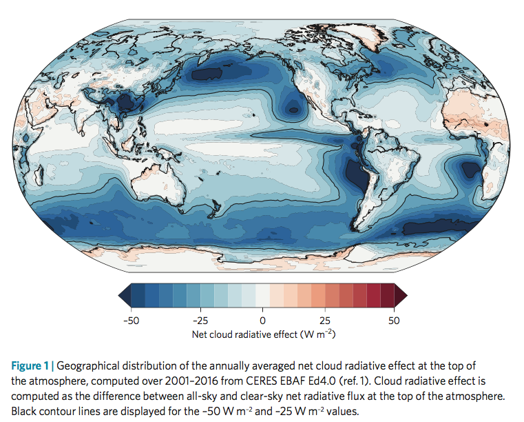
From Zelinka et al 2017
Figure 1 – Click to enlarge
Note that the cloud radiative effect shown above isn’t feedbacks from warming, it is simply the current effect of clouds. The big question is how this will change with warming.
In the next graphic, the inset in the top shows cloud feedback (note 1) vs ECS from 28 GCMs. ECS is the steady state temperature resulting from doubling CO2. Two models are picked out – red and blue – and in the main graph we see simulated warming under RCP8.5 (an unlikely future world confusing described by many as the “business as usual” scenario).
In the bottom graphic, cloud feedbacks from models are decomposed into the effect from low cloud amount, from changing high cloud altitude and from low cloud opacity. We see that the amount of low cloud is the biggest feedback with the widest spread, followed by the changing altitude of high clouds. And both of them have a positive feedback. The gray lines extending out cover the range of model responses.
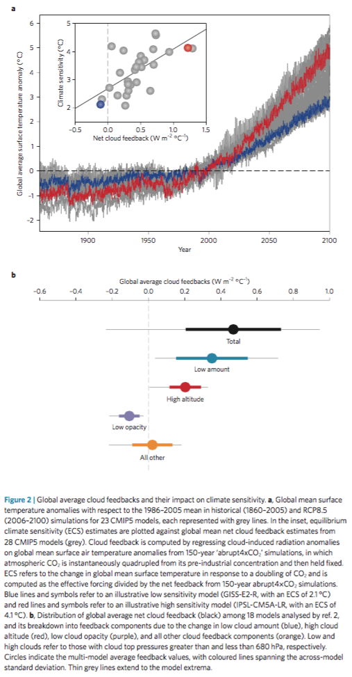
From Zelinka et al 2017
Figure 2 – Click to enlarge
In the next figure – click to enlarge – they show the progression in each IPCC report, helpfully color coded around the breakdown above:
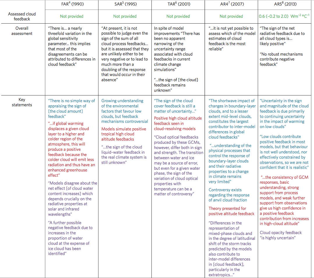
From Zelinka et al 2017
Figure 3 – Click to enlarge
On AR5:
Notably, the high cloud altitude feedback was deemed positive with high confidence due to supporting evidence from theory, observations, and high-resolution models. On the other hand, continuing low confidence was expressed in the sign of low cloud feedback because of a lack of strong observational constraints. However, the AR5 authors noted that high-resolution process models also tended to produce positive low cloud cover feedbacks. The cloud opacity feedback was deemed highly uncertain due to the poor representation of cloud phase and microphysics in models, limited observations with which to evaluate models, and lack of physical understanding. The authors noted that no robust mechanisms contribute a negative cloud feedback.
And on work since:
In the four years since AR5, evidence has increased that the overall cloud feedback is positive. This includes a number of high-resolution modelling studies of low cloud cover that have illuminated the competing processes that govern changes in low cloud coverage and thickness, and studies that constrain long-term cloud responses using observed short-term sensitivities of clouds to changes in their local environment. Both types of analyses point toward positive low cloud feedbacks. There is currently no evidence for strong negative cloud feedbacks..
Onto Ceppi et al 2017. In the graph below we see climate feedback from models broken out into a few parameters
- WV+LR – the combination of water vapor and lapse rate changes (lapse rate is the temperature profile with altitude)
- Albedo – e.g. melting sea ice
- Cloud total
- LW cloud – this is longwave effects, i.e., how clouds change terrestrial radiation emitted to space
- SW cloud- this is shortwave effects, i.e., how clouds reflect solar radiation back to space
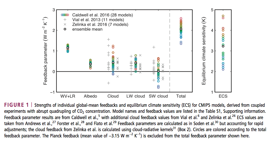
From Ceppi et al 2017
Figure 4 – Click to enlarge
Then they break down the cloud feedback further. This graph is well worth understanding. For example, in the second graph (b) we are looking at higher altitude clouds. We see that the increasing altitude of high clouds causes a positive feedback. The red dots are LW (longwave = terrestrial radiation). If high clouds increase in altitude the radiation from these clouds to space is lower because the cloud tops are colder. This is a positive feedback (more warming retained in the climate system). The blue dots are SW (shortwave = solar radiation). If high clouds increase in altitude it has no effect on the reflection of solar radiation – and so the blue dots are on zero.
Looking at the low clouds – bottom graph (c) – we see that the feedback is almost all from increasing reflection of solar radiation from increasing amounts of low clouds.
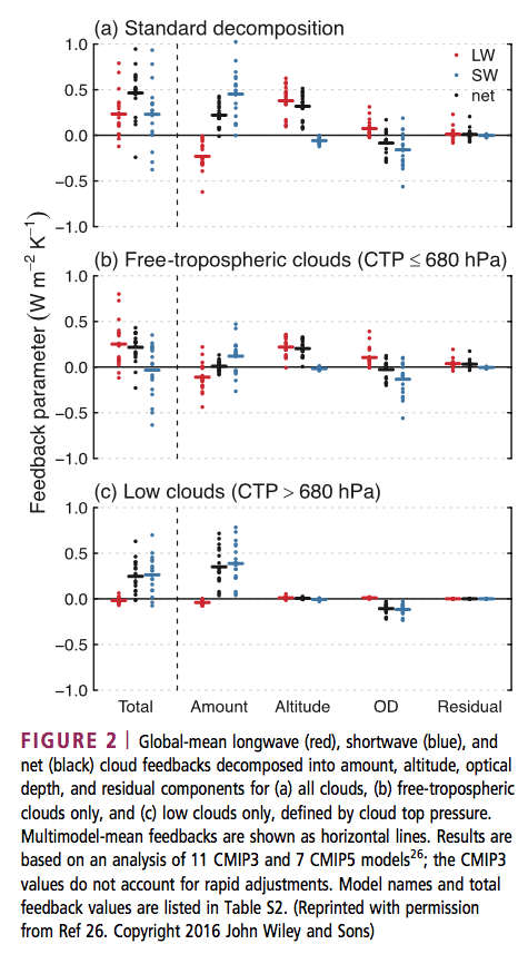
From Ceppi et al 2017
Figure 5
Now a couple more graphs from Ceppi et al – the spatial distribution of cloud feedback from models (note this is different from our figure 1 which showed current cloud radiative effect):
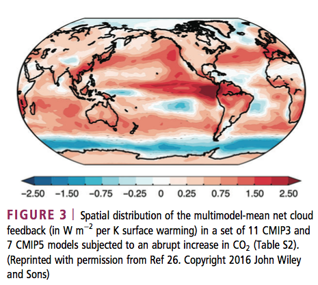
From Ceppi et al 2017
Figure 6
And the cloud feedback by latitude broken down into: altitude effects; amount of cloud; and optical depth (higher optical depth primarily increases the reflection to space of solar radiation but also has an effect on terrestrial radiation).
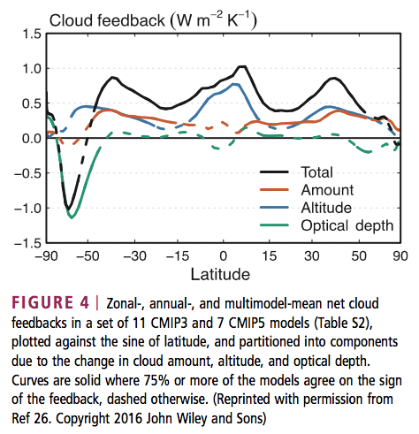
From Ceppi et al 2017
Figure 7
They state:
The patterns of cloud amount and optical depth changes suggest the existence of distinct physical processes in different latitude ranges and climate regimes, as discussed in the next section. The results in Figure 4 allow us to further refine the conclusions drawn from Figure 2. In the multi- model mean, the cloud feedback in current GCMs mainly results from:
- globally rising free-tropospheric clouds
- decreasing low cloud amount at low to middle latitudes, and
- increasing low cloud optical depth at middle to high latitudes
Cloud feedback is the main contributor to intermodel spread in climate sensitivity, ranging from near zero to strongly positive (−0.13 to 1.24 W/m²K) in current climate models.
It is a combination of three effects present in nearly all GCMs: rising free- tropospheric clouds (a LW heating effect); decreasing low cloud amount in tropics to midlatitudes (a SW heating effect); and increasing low cloud optical depth at high latitudes (a SW cooling effect). Low cloud amount in tropical subsidence regions dominates the intermodel spread in cloud feedback.
Happy Christmas to all Science of Doom readers.
Note – if anyone wants to debate the existence of the “greenhouse” effect, please add your comments to Two Basic Foundations or The “Greenhouse” Effect Explained in Simple Terms or any of the other tens of articles on that subject. Comments here on the existence of the “greenhouse” effect will be deleted.
References
Cloud feedback mechanisms and their representation in global climate models, Paulo Ceppi, Florent Brient, Mark D Zelinka & Dennis Hartmann, IREs Clim Change 2017 – free paper
Clearing clouds of uncertainty, Mark D Zelinka, David A Randall, Mark J Webb & Stephen A Klein, Nature 2017 – paywall paper
Notes
Note 1: From Ceppi et al 2017: CLOUD-RADIATIVE EFFECT AND CLOUD FEEDBACK:
The radiative impact of clouds is measured as the cloud-radiative effect (CRE), the difference between clear-sky and all-sky radiative flux at the top of atmosphere. Clouds reflect solar radiation (negative SW CRE, global-mean effect of −45W/m²) and reduce outgoing terrestrial radiation (positive LW CRE, 27W/m²−2), with an overall cooling effect estimated at −18W/m² (numbers from Henderson et al.).
CRE is proportional to cloud amount, but is also determined by cloud altitude and optical depth.
The magnitude of SW CRE increases with cloud optical depth, and to a much lesser extent with cloud altitude.
By contrast, the LW CRE depends primarily on cloud altitude, which determines the difference in emission temperature between clear and cloudy skies, but also increases with optical depth. As the cloud properties change with warming, so does their radiative effect. The resulting radiative flux response at the top of atmosphere, normalized by the global-mean surface temperature increase, is known as cloud feedback.
This is not strictly equal to the change in CRE with warming, because the CRE also responds to changes in clear-sky radiation—for example, due to changes in surface albedo or water vapor. The CRE response thus underestimates cloud feedback by about 0.3W/m² on average. Cloud feedback is therefore the component of CRE change that is due to changing cloud properties only. Various methods exist to diagnose cloud feedback from standard GCM output. The values presented in this paper are either based on CRE changes corrected for noncloud effects, or estimated directly from changes in cloud properties, for those GCMs providing appropriate cloud output. The most accurate procedure involves running the GCM radiation code offline—replacing instantaneous cloud fields from a control climatology with those from a perturbed climatology, while keeping other fields unchanged—to obtain the radiative perturbation due to changes in clouds. This method is computationally expensive and technically challenging, however.


The cloud feedback science of 2000 to 2007.
Joel Norris, Scripps Institution of Oceanography :
“cloud changes since 1952 have had a net cooling effect on the Earth”
“The decrease in reconstructed OLR since 1952 indicates that changes in upper-level cloud cover have acted to reduce the rate of tropospheric warming relative to the rate of surface warming. The increase in reconstructed net upward radiation since 1952, at least at middle latitudes, indicates that changes
in cloud cover have acted to reduce the rate of tropospheric and surface warming.”
“The surface-observed low-level cloud cover time series averaged over the global ocean appears suspicious because it reports a very large 5%-sky-cover increase between 1952 and 1997. Unless low-level cloud albedo substantially decreased during this time period, the reduced solar absorption caused by the reported enhancement of cloud cover would have resulted in cooling of the climate system that is inconsistent with the observed temperature record.”
It shows the climate science slowly retreating from former positions. So it is better to cling to models than to take observation seriously. It is possible that cloud cover was increasing for 45 years and has been decreasing a little the last 20 years. The whole 65 years span is most interesting, and maybe shows changes that are zero in sum.
My proposal for cloud feedback science, for global surface temperatures, base it on observation and statistics: Zero feedback is the best null hypothesis. Use climate models to test how different components can work together. Stop using models as speculative devices.
I think that I will correct myself here (after 4 years). It is now plenty of evidence of a global brightening, and that it was a “regime shift” about 1982. Shortwave radiation to earth surface increased, together with ocean heat content. It looks like changing clouds was responsible for much of the global warming from 1983 to 2021. The discussion of the part played by GHGs on this global brightening is not over.
I have some comments on clouds, longwave and shortwave feedback at the end of this comment serie.
It seems that when observations (IPCC) disagree with models, then the observations are assumed to be wrong, not the models.
I find it very odd that the pattern of positive cloud feedbacks from models clearly correlates with the measured net negative cloud effect from CERES. Seems to me we need a lot more measurement and a lot less modeling.
Steve,
Did you read the whole paper by Ceppi et al and follow up all the references?
Lots more measurement would be wonderful but in the meantime:
1. We only have 15 years of CERES measurements and we will only have 30 years of measurement we reach 2032. Perhaps we need 60 years of measurements which we will reach in 2062? On the other hand, if there is a way to get a better understanding before 2062 or 3032 wouldn’t you want that?
2a. There are lots of measurements apparently backing up the breakdown of cloud feedbacks, along with support from high resolution models. This is what Ceppi et al propose. So please address their points.
2b. GCMs compared with measurement compared with high resolution LES provide the opportunity to test hypotheses in more detail. You don’t want this? What would you propose as the alternative?
Yes, I read the article. It is a review article, with 181 references, most pay-walled. Are you suggesting that someone needs to read 181 references before commenting?
My take is the authors draw two apparently incongruent conclusions: 1) our understanding of cloud feedbacks in models has grown dramatically over the last 20 years, and 2) the models are no closer to agreeing with each other about cloud feedbacks than they were a dacade ago. And what do they propose? More research on this really hard problem. And better parameterizations of many processes below the model scale. And more ‘experiments’ with models using unrealistic conditions like instantaneous quadrupling of CO2. In other words, more of the same thing that has already been so effective over three decades at moving the models toward ever better agreement with each other and ever better consistency with measured reality. The contrast with Bjorn Stevens’ response to criticism of his paper on self-organization of convection could not be more clear: to paraphrase, “what we have been doing isn’t working, so we need a different approach”.
I am reminded by this review article of the presence of one recommendation in most all reports written by hired consultants: “you need more consulting”. My experience is that recommendation is often very wrong, and I don’t think that should come as a surprise to anyone. (I worked as a technical consultant for more than 15 years.)
If CERES measurements are useful, then we should be able to see clear trends over 15 years, and certainly over 30 years. If the data are too noisy/uncertain to provide meaningful confirmation of model projections (e.g., the patern of global radiative balance has seen a clear and significant trend, just as predicted by models), and to tell us which models, get clouds “right” and which get them “wrong”, then yes, we need more and/or better data…. as much as it takes. Progress is never made doing what you already know doesn’t work.
Yes, the models have gotten quite a bit better at matching reality and in agreeing with each other over the last three decades. They have objectively improved on many metrics, and do a much better job of representing smaller-scale phenomena than they used to. So, it seems wise to continue this.
Even if there was still the same amount of disagreement within models, though, that doesn’t mean you abandon them. Models, as the representation of our knowledge of how a system works, are the ultimate goal of any science. It doesn’t always have to be computer models, but the goal is still to understand reality through simplified conceptual models. This is the same guiding principle across every field.
So we keep improving our conceptual understanding of how the Earth’s climate system works. That goes hand-in-hand with improving our models; the conceptual understanding is the same whether or not you’ve programmed it into a computer.
I ask myself this question:
– we can always point to the deficiencies of a model (or a group of models)
– this is because all models are wrong – although some are useful
So at what point do we find model results useful? Never?
Models are generally useful when they make accurate predictions over a significant period of time. (That is, more accurate than a simple extrapolation of recent history.) Model predictions used to justify huge public and private costs, everywhere on Earth, have to 1) agree closely with each other, and 2) make remarkably accurate predictions, not hind-casts, over multi-decadal periods. Neither of these are close to the state of GCMs.
SOD asked: “So at what point do we find model results useful? Never?”
For me, when the models reproduce the large changes in OLR and OSR from clear and cloudy skies that accompany the seasonal cycle of warming – without having been tuned to do so. Hopefully, the agreement will be regional as well as global.
I ask myself in what way climate models are useful. This is a perturbed physics ensemble from Rowland et al 2012. It is conveniently compared to the CMIP opportunistic ensemble. The claim is an even broader range of outcomes.
The 1000’s of solutions in the perturbed physics ensemble diverge exponentially as a result of sensitive dependence on initial conditions – and the spread is ‘irreducible imprecision’. Sensitive dependence and structural instability are intrinsic properties of climate models resulting from the nonlinear nature of the core equations of fluid transport.
“Lorenz was able to show that even for a simple set of nonlinear equations (1.1), the evolution of the solution could be changed by minute perturbations to the initial conditions, in other words, beyond a certain forecast lead time, there is no longer a single, deterministic solution and hence all forecasts must be treated as probabilistic. The fractionally dimensioned space occupied by the trajectories of the solutions of these nonlinear equations became known as the Lorenz attractor (figure 1), which suggests that nonlinear systems, such as the atmosphere, may exhibit regime-like structures that are, although fully deterministic, subject to abrupt and seemingly random change.” Slingo and Palmer 2011
The implications for opportunistic ensembles are profound. Non-unique solutions from different models are compared without questioning the theoretical basis for individual solution choice. It is done on the basis of a posteriori solution behavior – i.e. the solution looks good without having any rigorous basis for the choices made.
We do of course have regime like shifts in oceans and atmosphere. One of these is of course the ENSO quasi standing wave in the globally coupled, spatio-temporal chaos of Earth’s flow field. ENSO origins are in upwelling in the eastern and central Pacific. This is influenced by blocking patterns spinning up ocean gyres in the north and south in response to polar surface pressure changes. Models are linking polar surface pressure changes to solar UV/ozone chemistry – intrinsically a better role for models in process formulation. e.g. https://www.nature.com/articles/ncomms8535
The significance for cloud is in the response to changing sea surface temperature – for which there is theoretical – e.g. http://aip.scitation.org/doi/abs/10.1063/1.4973593 – and both surface and satellite observation – e.g. – http://science.sciencemag.org/content/325/5939/460 – http://journals.ametsoc.org/doi/pdf/10.1175/JCLI3838.1 – but the future of sea surface temperature is unknowable. It seems a relatively large effect and ENSO shows extreme variability over many millennia.
“Figure 12 shows 2000 years of El Nino behaviour simulated by a state-of-the-art climate model forced with present day solar irradiance and greenhouse gas concentrations. The richness of the El Nino behaviour, decade by decade and century by century, testifies to the fundamentally chaotic nature of the system that we are attempting to predict. It challenges the way in which we evaluate models and emphasizes the importance of continuing to focus on observing and understanding processes and phenomena in the climate system. It is also a classic demonstration of the need for ensemble prediction systems on all time scales in order to sample the range of possible outcomes that even the real world could produce. Nothing is certain.” op. cit.
A news release about the Ceppi paper.
STUDY DISCOVERS WHY GLOBAL WARMING WILL ACCELERATE AS CO2 LEVELS RISE
SOD and Steve, Let me make a few points:
1. A recent paper Zhao et al on a new GFDL GCM makes the following point — “The authors demonstrate that model estimates of climate sensitivity can be strongly affected by the manner through which cumulus cloud condensate is converted into precipitation in a model’s convection parameterization, processes that are only crudely accounted for in GCMs. In particular, two commonly used methods for converting cumulus condensate into precipitation can lead to drastically different climate sensitivity, as estimated here with an atmosphere–land model by increasing sea surface temperatures uniformly and examining the response in the top-of-atmosphere energy balance. The effect can be quantified through a bulk convective detrainment efficiency, which measures the ability of cumulus convection to generate condensate per unit precipitation. The model differences, dominated by shortwave feedbacks, come from broad regimes ranging from large-scale ascent to subsidence regions. Given current uncertainties in representing convective precipitation microphysics and the current inability to find a clear observational constraint that favors one version of the authors’ model over the others, the implications of this ability to engineer climate sensitivity need to be considered when estimating the uncertainty in climate projections.” This is I think alarming in terms of relying on GCM’s for future projections.
2. Nic Lewis makes the following point regarding GCM predicted cloud fraction by latitude — “Even if the CMIP5 average water vapour + lapse rate feedback of ~1.0 Wm−2 °C−1 were correct, combining it with the Planck and albedo feedbacks would only generate an ECS of ~2°C, much lower than the diagnosed ECS values of the CMIP5 models used to generate projections of warming over this century, which average 3.4°C. The difference relates primarily to positive cloud feedbacks in AOGCMs. Clouds are unresolved sub-grid scale phenomena in AOGCMs and are represented by parameterized approximations. Clouds at different levels have very different effects. Low clouds generally cool the Earth by reflecting incoming short-wave solar radiation, whilst having little effect on outgoing long-wave radiation (although they are opaque to long- wave radiation, most of it that leaves Earth is emitted higher in the atmosphere). High level, thinner, clouds generally warm the Earth by transmitting most short-wave radiation, but blocking outgoing long-wave radiation. Current models do not even succeed in representing basic features such as total cloud extent at all accurately, as this graph comparing percentage total cloud fraction in CMIP5 AOGCMs with that per satellite observations shows:” [unfortunately pasting the plot is beyond my meager computer skills, but you can find it at Nic’s web site.]
3. Convection, the main cloud generating phenomenon in the tropics, is an ill-posed problem. It is unlikely in my view that current low resolution GCM’s will get much right here beyond a small number of outputs which can be used to tune the parameters. As shown in 1 however, these processes can have a very large effects on the ECS of a GCM. At the least, this points to a huge gap in our understanding of what to tune and how one can meaningfully constrain GCM outputs of interest to policy makers.
dpy6629,
For interested readers, we had a look at a similar paper – Cloud tuning in a coupled climate model: Impact on 20th century warming, Jean-Christophe Golaz, Larry W. Horowitz, and Hiram Levy II, GRL (2013) – in Models, On – and Off – the Catwalk – Part Five – More on Tuning & the Magic Behind the Scenes and then in the comments also discussed Zhao et al.
I’m looking forward to digging through the papers referenced by Ceppi et al to see how well LES models match up with observations and how well both match up on the FAT (fixed anvil temperature) hypothesis, the low cloud amount and other cloud feedbacks.
One of the papers I was just reading (probably a Ceppi reference) made this same point and we can also see it in figure 4 in the article.
Do you have a link?
The Nic Lewis quotation comes from: Equilibrium Climate Sensitivity and Transient Climate Response – the determinants of how much the Earth’s surface will warm as atmospheric CO2 increases, point 21.
The best I have SOD is this from Nic Lewis. In my experience he is very reliable in reporting others findings.
Click to access briefing-note-on-climate-sensitivity-etc_nic-lewis_mar2016.pdf
See particularly the later points.
Well good luck with the LES modeling. Here’s a rare papers on grid sensitivity of DES, which uses LES in the separated flow regions away from the wall.
https://arc.aiaa.org/doi/full/10.2514/1.J055685
I still wonder what rigorous methods one can use to assess the accuracy of these methods. You are aware that LES results will be dependent on grid density so grid convergence is very challenging.
In any time accurate turbulent simulation, the adjoint diverges and this fact makes classical numerical error control methods impossible. In the absence of numerical error control, it seems to me problematic to separate the numerical noise from the signal.
I would be quite interested in any alternatives you uncover in your reading.
The graph referenced in point 21 was taken from Propagation of Error and The Reliability of Global Air Temperature Projections – Patrick Frank
JCH,
In that case the graphic is this one:
SOD, I value highly your posts on recent papers like this one. It’s always informative and interesting and I thank you for your work. It’s a great forum for learning about climate science.
However, perhaps what SteveF is frustrated by is how uncertain a lot of the results are given the poor quality of the data and the models. I recently was investigating something I saw elsewhere on the web and it led me to a RealClimate post about a 2005 Nature paper stating that “high aerosol forcing will mean much more warming in the future.” This paper was raising the possibility that ECS could be as high as 10C if aerosol forcing was say -2W/m2. Schmidt’s post was basically debunking that paper.
http://www.realclimate.org/index.php/archives/2005/07/climate-sensitivity-and-aerosol-forcings/
The reason it was interesting to me was the graphics of ECS vs. total aerosol forcing based on a simple energy balance model that foreshadowed some of Nic Lewis’ work. Unfortunately, the original RealClimate post does not have the graphs probably due to data storage limitations, but I found it elsewhere and indeed according to Schmidt’s graphic if total aerosol forcing is around -1.0 W/m2, ECS is about 1.5C.
In any case, there are many more examples of “alarming” papers that say its going to be much worse than we thought that turn out to be of low quality.
The other point I would make SOD is that it is wise to exercise skepticism with regard to the literature in a politically charged field like climate science. I know in CFD that the literature is untrustworthy because most of it suffers from selection bias. People want to keep their funding stream alive so they tend to “select” their “best” results and file in the desk drawer the less convincing results. The bad results can always be explained as due to bad griding, numerical instabilities, unconverged iterations, and finally if you are brazen you can claim the data must be wrong. This is equivalent to rounding up and burning the usual witches when things don’t work as you would want.
I believe that in climate science there is a group of activist scientists who are reluctant to publish results that are not alarming. The best example of this is the IPCC redoing an energy balance paper’s calculations using a uniform prior in its chapter on ECS. That of course led to a much higher estimate than the original paper. That’s why Lewis is so valuable in this field.
dpy6629,
In this blog – check the Etiquette – we ignore presumed motivations.
The ideas in the Etiquette and in About this Blog are the principles behind the blog. There are much better blogs to debate the motivations, nefarious activities and subconscious plotting of climate scientists.
But not here.
Instead, commenters should limit themselves to presenting evidence against (or for) a point of view.
OK, sorry. I’ve seen this myself in CFD where the bias is not usually intentional. There are always rationalizations and the culture tends to provide its own survival imperative. As in any field, some people are vastly worse than others. This can be a function of personality. There is plenty of this bias in all fields of science.
SOD: I haven’t studied the material above carefully enough, but I everything appears to be comparing models to models. Let’s compare models to observations: The change in OLR and reflected SWR (OSR) from both clear and cloudy skies associated with the 3.5 K of seasonal warming the planet undergoes every year. This arises from an average of about 10 K of warming in the NH (with its lower heat capacity responding to seasonal increased irradiation) and 3 K of cooling in the SH. Unfortunately, the data is reported in terms of gain factors not W/m2/K. A gain factor of f will increase the no-feedbacks climate sensitivity by a factor of (1/(1-f)).
The gain factors of longwave feedback that operates on the annual variation of the global mean surface temperature. (A) All sky. (B) Clear sky. (C) Cloud radiative forcing. Blank bars on the left indicate the gain factors obtained from satellite observation (ERBE, CERES SRBAVG, and CERES EBAF) with the SE bar. Black bars indicate the gain factors obtained from the models identified by acronyms at the bottom of the figure (Methods, Data from Models). The vertical line near the middle of each frame separates the CMIP3 models on the left from the CMIP5 models on the right.
The gain factors of solar [reflected SWR] feedback that operate on the annual variation of the global mean surface temperature. (A) All sky. (B) Clear sky. (C) Cloud radiative forcing. See Fig. 3 legend for further explanation.
The evidence is undeniable that AOGCM’s have serious problems reproducing the large changes that are seen annually in response to the seasonal 3.5 K increase in GMST – except for an LWR feedback of about -2.1 W/m2/K through clear skies (Planck+WV+LR). Most models show LWR feedback from all skies that is more positive than observed.
Until AOGCMs are capable of better reproducing these seasonal feedbacks, why should we pay any attention to model vs. models comparisons? Why does anyone believe we can learn anything from comparing one flawed model to another? (Are climate models tuned to produce LWR feedback in response to seasonal warming of about -2.1 W/m2? If not, then this is something they get right.)
———————————
The strongly positive SWR gain factors observed with seasonal warming may not be relevant to global warming. The error bars are much larger because reflection of OSR (unlike LWR) doesn’t change linearly with monthly Ts. Some changes are lagged, particularly sea ice, which has a minimum in September and a maximum in March in the NH and the opposite in the SH. The composite has two maxima during summer in the NH: the larger in September and the second several months earlier. The SH has very little land covered by seasonal snowfall. So feedbacks in OSR observed through clear skies during seasonal warming may have nothing to do with ice-albedo feedback in global warming.
The monthly change in OSR from cloudy skies is also not very linear with temperature and appears to have lagged relationships. So observations tel us that climate models represent important seasonal feedbacks very poorly, but they don’t tell us what feedbacks will accompany global warming (except perhaps clearly sky LWR feedback: Planck+WV+LR).
In my own field (materials science), there’s quite a bit you can learn from comparing one flawed model to another. It helps you understand how changing the underlying parameters, or gridding, or numerical scheme, etc., can change the results.
Basically, it’s an exploration of parameter space. It adds to our understanding of how things work; how varying this fundamental parameter changes that derived one.
It looks like there’s a fair amount of disagreement even among the observations. CERES EBAF differs from the other two by a not-insubstantial amount.
If cloud feedback is net strongly negative now, but increases in cloud cover will cause positive feedback, then one would assume that increasing cloud cover from zero to x%, where x is less than 30, must have strong initial negative feedback change per percent cover which declines as cloud cover increases and becomes positive at some point less than 30% cover. It’s not at all clear to me how this would work. It’s also not clear to me that 100% cloud cover would result in a warmer planet. The nuclear winter folks didn’t think so, not that they were particularly believable.
So let’s say that the cloud cover fraction doesn’t change, but the location and cloud top altitude changes as a result of warming result in less negative feedback. The problem here is that cloud cover data in models is wrong now. Why should we believe that the model predictions of trends when starting from the wrong initial conditions will somehow be correct? As I’ve said before, just because researchers haven’t found a strongly negative cloud feedback model doesn’t mean there isn’t one.
Some systematical bias in models:
“Abstract: The Cloud-Aerosol Lidar and Infrared Pathfinder Satellite Observation (CALIPSO) satellite provides robust and global direct measurements of the cloud vertical structure. The GCM-Oriented CALIPSO Cloud Product is used to evaluate the simulated clouds in five climate models using a lidar simulator. The total cloud cover is underestimated in all models (51% to 62% vs. 64% in observations) except in the Arctic. Continental cloud covers (at low, mid, high altitudes) are highly variable depending on the model. In the tropics, the top of deep convective clouds varies between 14 and 18 km in the models versus 16 km in the observations, and all models underestimate the low cloud amount (16% to 25%) compared to observations (29%). In the Arctic, the modeled low cloud amounts (37% to 57%) are slightly biased compared to observations (44%), and the models do not reproduce the observed seasonal variation.”
From: About the observation of cloud changes due to greenhouse warming
Hélène Chepfer 2014
Click to access CERES-ScaraB-GERB-Toulouse-Oct2014.pdf
Let us sum up models vs observation:
The total cloud cover is underestimated except in the Arctic.
The low cloud amount is underestimated compared to observations.
Models do not reproduce the observed seasonal variation.
I would not think that these five climate models have less systematical bias than other models. But I find it difficult to dig out such data.
Other papers find that it hasn`t been any decrease in cloud cover the last 25 years (perhaps with the exception of some change in distribution). Or even over 60 years (Eastman et al. 2011)
JCH,
Or it could be related to a multi-decadal cycle. We won’t know for another few decades.
Observed cloud cover: “Overall, most of the studies reviewed suggest an increase in the TCC since the late 19th century, and in particular from the early until the mid/late-20th century, both over land and ocean. Although possible artifacts in these trends cannot be ruled out, it seems difficult to argue that these possible biases in the observations could explain the significant increases observed worldwide,” TCC is total cloud cover.
For Spain, which is the object of the study: “The linear trend for the annual mean series, estimated over the 1866–2010 period, is a highly remarkable (and statistically significant) increase of +0.44 % per decade, which implies an overall increase of more than +6 % during the analyzed period. These results are in line with the majority of the trends observed in many areas of the world in previous studies, especially for the records before the 1950s when a widespread increase of TCC can been considered as a common feature.”
From:Increasing cloud cover in the 20th century: review and new findings
in Spain. A. Sanchez-Lorenzo, J. Calbo´ and M. Wild, 2012
Yes, and that is why I noted the clear correlation between the pattern of current net cooling from clouds and the model projected net warming effect from changes in cloud cover. We are supposed to believe clouds cause strong net cooling at present, but less strong net cooling in the future, with the pattern in the projected drop in net cooling closely following the pattern of current net cooling due to clouds. Which indicates there is a “goldielocks” fraction of cloud cover which maximizes net cooling… any more or any less reduces net cloud cooling. Seems to me quite a stretch. Some might say “implausible”.
Sorry, the above comment was a reply to DeWitt’s comment.
I don’t think so. If you’re just increasing the cloud cover (keeping the same ratios of types of clouds), then I’d expect that the net cooling would continue to increase.
It’s more that the type / altitude / location of clouds changes. You aren’t just keeping the cloud types the same.
So I’m not really following you. I’m not sure why there couldn’t be local maxima in the cooling effects of clouds; why the cloud feedbacks can’t switch sign. Do you have more reasoning behind this?
Windchaser,
“Do you have reasoning behind this?”
Of course.
As DeWitt pointed out above: “The problem here is that cloud cover data in models is wrong now.” It is not like the models are so damned accurate about cloud cover that it beggars belief, it is quite the opposite: they are so damned inaccurate that it beggars belief. (see the Nic Lewis graph of cloud cover posted by SoD above on December 27)
You have a bunch of models which broadly disagree with each other about cloud feedbacks, are “no closer to agreement than a decade ago” about cloud feedbacks, and which generate, both individually and on average, a clearly inaccurate pattern of cloud cover when compared to measured cover. Considering that cloud feedbacks in GCMs represent a big fraction (most?) of the difference between empirical and GCM estimates of sensitivity (~1.9C vs ~3.4 C per doubling), there seems to me plenty of reason to doubt model projections of future cloud changes. If the models are correct about how warming changes cloud cover, that should already be clear in CERES data; it’s not.
Not saying the graph is wrong, but it came from what I believe is called a poster at an AGU convention. Are they peer reviewed?
JCH,
Not as far as I know. I think, however, you may have entirely too much faith in the screening capability of the peer review system. I wouldn’t take a peer reviewed paper as gospel. I think the credibility level of a poster at a major conference would be about the same as for a peer reviewed paper in an average journal. The level of skepticism should be similar.
But even the major journals can publish questionable science. See, for example, Steig, et. al., 2009 cover article in Nature about the pattern of warming in Antarctica since 1957:
https://www.nature.com/articles/nature07669
That was found to have significant errors by O’Donnell, et. al., 2010
http://journals.ametsoc.org/doi/abs/10.1175/2010JCLI3656.1
The authors had a difficult time getting their paper published because, apparently, Steig was one of the reviewers.
DeWitt,
“The authors had a difficult time getting their paper published because, apparently, Steig was one of the reviewers.”
There is no ‘apparently’ involved; Eric Steig was the reviewer who demanded the authors not claim Steig et al was wrong.
I think, however, you may have entirely too much faith in the screening capability of the peer review system.
Dewitt – I view peer review as a ticket to a more comprehensive review and nothing more than that. It obviously does not mean the paper is error free or advances the science in any way, which has to be a major goal of the exercise: advancement.
In the case of Steig09 and the subsequent O’Donnell et al paper, perhaps I am wrong, but I suspect there is an almost zero likelihood that any of the authors of O’Donnell paper would ever in their entire lives written a paper about temperature trends in Antarctica if not for Steig09. Sounds like science was advanced.
JCH,
The history of O’Donnell at al is actually interesting. After the Steig Nature paper (with the image of a uniformly warming Antarctica on the cover), O’Donnell, Jeff Condon, McIntyre, and others commented on the Realclimate web site, where Steig had posted a writeup, and said that the reconstruction didn’t look right (for a number of reasons, including obvious discrepancies with ground station data). Despite offering clear explanations of what was wrong, Ryan O’Donnell, Jeff Condon and others were dissed by the Realclimate crew, who said they didn’t know what they were talking about. What those folks at Realclimate did not know was that O’Donnell was very familiar with the type of ‘inverse’ problem in Steig et al, and could see that they were mathematically smearing warmth from the peninsula region over the whole continent. In the end Steig pretty much told them to go write their own paper and stop wasting his time. That was a mistake. Yes, science ultimately advanced (people finally understood that most of Antarctica was not actually warming rapidly) but it could have been a lot quicker, easier, and less contentious had Steig at al been willing to listen.
JCH quoted: “Here we show that several independent, empirically corrected satellite records exhibit large-scale patterns of cloud change between the 1980s and the 2000s that are similar to those produced by model simulations of climate with recent historical external radiative forcing.
What does the phrase “independent, empirically-corrected satellite records” actually mean? It means that the roughly 3% reduction in ISCCP cloud cover observed since 1985 is removed by empirical correction – ie corrections without any physical rational. It means elimination of most of the variability in PATMOS cloud cover (which is as big as ISCCP variability, but not a gradual reduction). Any variability that correlates with satellite zenith angle or sun angle (equatorial crossing time) is eliminated using a different fit for each grid cell. And any variability that might be attributed to artifacts from a single geostationary satellite is removed. All of these corrections are hypotheses that have been not been tested. The authors say:
“Note that any real variability in cloud fraction that happens to be correlated with variability in artifact factors will be removed by our correction procedure, but we consider a corrected dataset with some real variability removed preferable to a dataset with no real variability removed but dominated by artifacts.”
http://journals.ametsoc.org/doi/10.1175/JTECH-D-14-00058.1
According to the multi-model CMIP5 mean, anthropogenic factors should have caused changes of up to +/-0.5 to 1.0% in cloud cover over the last 25 years in some grid cells. The observed change in cloud cover in some grid cells is greater than 3%. If the corrected observations and models agree in trend direction, that is called agreement.
The data suggesting that cloud top heights in the tropics have risen may be somewhat more robust, but we are still talking about changes of about 0.5% over 25 years.
Then one still faces the issue of converting changes in cloud amount and cloud altitude with warming into changes in OLR and OSR.
Above, I asked why anyone would pay attention to this noisy, inconclusive data when we have very clear evidence from the seasonal cycle that LWR cloud feedback is slightly negative, not positive as most models predict? And there is no consensus among models about seasonal SWR cloud feedback.
The paper has been cited 58 times. I went through all of the ones cited that have complete copies available. The scientists who have cited it appear to be in the forefront of research to do with clouds. One was cited in opposition above. He used a result of this study in recent work. Stevens has a goal.
Frank asked: “Why anyone would pay attention to this noisy, inconclusive data (Norris 2016) when we have very clear evidence from the seasonal cycle that LWR cloud feedback is slightly negative, not positive as most models predict (Tsushima and Manabe 2013)? And there is no consensus among models about seasonal SWR cloud feedback.”
JCH replied: “The paper has been cited 58 times”, and reviewed the background of those citing the work.
Tsushima and Manabe 2013 has been cited only 4 times, despite the fact that Syukuro Manabe is one of the most respected figures in climate science. None of these citations endorsed the conclusion of this paper: Three appear to be large review articles and the fourth was an E&E paper that claims ECS is about 0.15K (that has only been cited once by its own author). Could this be because Norris 2016 says observations of clouds agree with models while Tsushima and Manabe 2013 say models are biased (and their data shows they are mutually inconsistent)?
Immediately below is the data that defines LWR feedback during seasonal warming. I challenge anyone to show me another climate science paper with tighter observational data. This is because you are looking at the biggest temperature change and seasonal warming has been observed once a year for the last thirty years. I posted the results for models above.
The globally averaged, monthly mean TOA flux of outgoing longwave radiation (Wm−2) over all sky (A) and clear sky (B) and the difference between them (i.e., longwave CRF) (C) are plotted against the global mean surface temperature (K) on the abscissa. The vertical and horizontal error bar on the plots indicates SD. The solid line through scatter plots is the regression line. The slope of dashed line indicates the strength of the feedback of the first kind [Planck feedback alone]. [The values on the y-axis represent heat lost and technically should have a negative sign.]
I don’t have the ability to paste figures from Norris (2016), but the observed change in cloud coverage shows changes 3-5X those predicted by climate models (See vertical scale.) Some other caveats:
“This is because observational systems originally designed for monitoring weather have lacked sufficient stability to reliably detect cloud changes over decades unless they have been corrected to remove spurious artifacts.”
“Note that any real variability in cloud fraction that happens to be correlated with variability in artifact factors will be removed by our correction procedure, but we consider a corrected dataset with some real variability removed preferable to a dataset with no real variability removed but dominated by artifacts.”
Worst of all, Norris (2016) tells us that models qualitatively agree with highly processed observations, but I doesn’t tell us anything quantitative about cloud feedback.
So why does a study that definitively shows AOGCMs are biased (and mutually inconsistent) get no significant citations in more than 4 years while Norris has 58 citations in 1.5 years.
Our host dislikes speculation about motivations. So I’ll simply ask: “Without AOGCMs, what does climate science have to offer policymakers?
Frank,
“Without AOGCMs, what does climate science have to offer policymakers?”
Well, there is broad consensus that equilibrium climate sensitivity is unlikely to be less than 1.5C per doubling, and transient sensitivity unlikely to be less than 1C. It is therefore possible to give policymakers (in democracies, that would ultimately be us!) lower bound estimates for future warming for any projected rise in CO2, and (at least in theory) make lower bound estimates of future costs and benefits. Unfortunately “future costs and benefits” are as often as not subject to wildly differing estimates, because of both the complexity of making projections, and because people assign very different ‘values’ to the same actual outcome… eg. What is the “cost” of having a 33% lower population of polar bears? (assuming that was a quantifiable outcome)
Frank,
So why does a study that definitively shows AOGCMs are biased (and mutually inconsistent) get no significant citations in more than 4 years while Norris has 58 citations in 1.5 years.
The reason the Norris paper has a high number of citations is that it is introducing a useful dataset. They get a citation whenever anybody uses that dataset.
Why doesn’t Tsushima and Manabe 2013 have more citations? We’d really need to question why it would be cited to understand that.
You seem to be impressed that the paper demonstrates biases in GCMs but actually that’s been done in hundreds, even thousands, of other papers. Just type “cloud biases GCMs” into google scholar for a subset.
In terms of the technique they propose for quantifying cloud and radiation biases based on seasonal cycle variations, this 2013 paper is really just rehashing one from the same authors from 2005, which has been cited 22 times according to the journal (38 times according to google). However, this seems to have been fairly quickly outdone in terms of model error quantification methods in the climate science world by Gleckler et al. 2008, which has 360 (674) citations and provided the methodological basis for much of the demonstration of model biases in IPCC AR5 Chapter 9.
In terms of a seasonal cycle cloud bias assessment being applied to the latest generation of CMIP models, this paper was already outdone by one published a few months earlier by the same lead author. It has been cited 20 (30) times, including numerously by AR5 Chapter 9. Tsushima and Manabe 2013 seems to have been a bit of a highlights reel spin off from that more substantial assessment.
Ultimately there doesn’t seem to be a great reason for citing that paper because it doesn’t bring anything new to the table.
Thank you for the presentation of Tsushima and Manabe, Frank.
I find it very convincing. It doesn`t only show model bias and spread, but it also shows that models get it systematically wrong. And it will be hard for many scientists to admit, when they are invested in their beliefs about clouds positive feedback, and when they keep repeating that models get reality reasonable right.
Paulski0: Thank you so much for the extremely responsive and useful answer. I just started trying to digest the Tsushima 2012 Climate Dynamics paper (T12). Some initial comments. TM13 is about feedback (W/m2/K), and therefore climate sensitivity. It uses our most reliable observational data (TOA OLR and OSR) and all CMIP3 and 5 models. T12 is about a variety of cloud observations (W/m2, % coverage, etc.) and a handful of CMIP5 models. It doesn’t bear directly on climate sensitivity.
Those using and citing the empirically corrected cloud data set should be citing Norris (2015) and have done so 34 times in 2.5 years. Those citing the conclusion that the corrected data set agrees with model predictions should be citing Norris (2016) and have done so 58 times in 1.5 years.
For me, TM13 clearly illuminates some important facts about seasonal feedbacks, which useful models should reproduce. Models are clearly mutually inconsistent in their predictions about OLR and OSR from clear and cloudy skies. Overall climate feedback parameters may agree, but only because of compensating errors. On the monthly time scale, OLR is a tight function of Ts (2.1 W/m2/K), with a slightly negative CRE. Most AOGCMs have a positive CRE and some are badly wrong. Models don’t properly reproduce seasonal changes in OSR, but these are not a tight function of Ts. Some component probably lag; others may be caused by hemispheric differences (in seasonal snow cover, sea ice and geography). Applying the gain factors TM13 calculate to global warming is problematic.
I need to stop talking and see what the other references you provide say about these important (and possibly ignored) conclusions.
I find it very convincing. It doesn`t only show model bias and spread, but it also shows that models get it systematically wrong. And it will be hard for many scientists to admit, when they are invested in their beliefs about clouds positive feedback, and when they keep repeating that models get reality reasonable right.
I guess Manabe is one who you think finds something too difficult to admit. Weird interpretation. He cowrote the paper. Frank wants to use the paper to imply that models are wrong, and Manabe’s early model cannot fairly be described by the word “wrong”:
JCH wrote: “I guess Manabe is one who you think finds something too difficult to admit. Weird interpretation. He cowrote the paper. Frank wants to use the paper to imply that models are wrong, and Manabe’s early model cannot fairly be described by the word “wrong”:
FWIW, the ECS of M&W 1967 model was 2.0 K. That may explain why you say his early projection was about right, why the central estimates for EBMs are 1.5-2.0 K, and why the OLR gain factor observed in T&M13 is consistent with an ECS of 1.8 K.
Manabe doesn’t inform us (in the limited space provided by PNAS) that OSR has some components that lag monthly Ts (see scatter plot) and some components that reflect hemispheric differences. (For example, there is negligible seasonal snow cover in the SH to reflect SWR through clear skies). Therefore, the OSR gain factor for the seasonal cycle is not directly relevant to global warming. However, it is a reasonable criteria for identifying biases in models. Spenser and Lindzen&Choi have both found that the best correlation between OSR and Ts involves a three-month lag and shifts from positive feedback with zero lag to negative feedback. L&C found this in the tropics, so it is not simply a problem involving surface (ice) albedo feedback. I personally disagree with using either zero or three month lag; I think the data is saying that OSR is not a simple function of Ts at any particular time. (Temperature controls emission of OLR, but reflection of SWR is obviously far more complicated.)
Manabe’s abstract diplomatically concludes: “we show that the gain factors obtained from satellite observations of cloud radiative forcing are effective for identifying systematic biases of the feedback processes that control the sensitivity of simulated climate, providing useful information for validating and improving a climate model.”
Is Manabe implying that AOGCMs need validation? That they failed validation?
I would go a little further: The data clearly shows that models are seriously mutually inconsistent. I don’t know what Manabe believes about the utility of a multi-model mean of mutually-inconsistent models. If he had shown the data, the LWR gain factor for the multi-model mean would be too high, inflating ECS and projected warming.
As the saying goes: “All models are wrong; some models are useful.” The question is whether current models are useful for informing policymakers about the likelihood that ECS is greater than 2 K. The IPCC and the climate science community have totally ducked their responsibility for presenting this issue in their Summaries for Policymakers and to the public.
Frank,
If he had shown the data, the LWR gain factor for the multi-model mean would be too high, inflating ECS and projected warming.
Except the LWR gain factors shown do not correlate at all with the models’ climate sensitivities. The highest gain is from one of the lower sensitivity models and the lowest gain is from one of the higher sensitivity models. In fact the alternative version of that latter model has a markedly reduced sensitivity but shows higher gain. So, while the test may provide a useful pointer to model biases it doesn’t carry any clear implication for climate sensitivity.
For similar tests which do appear to correlate with climate sensitivity, generally it has been found that higher sensitivity models show smaller biases. That’s the basis of the recent Brown and Caldeira paper and also a conclusion from the 2012 Tsushima paper: ‘The models in this study that best capture the seasonal variation of the cloud regimes tend to have higher climate sensitivities.’
DeWitt,
Your argument I think is only valid if feedback is quoted as vs cloud cover fraction.
It isn’t; it’s quoted vs temperature.
I don’t think the absolute value of cloud forcing in principle tells you anything at all about how it will change with respect to temperature.
vtg,
Yes, probably.
However, I think there may be confusion in cause and effect on location of cloud cover and surface temperature. I’m thinking now that a possible mechanism for the apparent multi-decadal oscillation in temperature in the surface record that is highly correlated with the AMO Index data might be changes in the pattern of cloud cover possibly driven by shifts in ocean currents that are chaotic in nature rather than driven solely by increases in anthropogenic ghg’s. Inherently chaotic processes can produce oscillatory behavior, at least for a while. We also know there was a major shift in the North Atlantic around 1995. That’s when Arctic Sea ice loss accelerated. I can also see what looks like a break point around that date in the UAH NoPol TLT temperature data.
Two of the model trends in response to warming seem reasonable: convective cloud tops in tropics increase in height, non-convective cloud belts shift northwards into areas with lower sun angles.
Reply to Paulski0. Thanks for the Glecker reference. A very interesting paper that. And happy New Year to all!
What you’ve highlighted here is really a very interesting part of climate science. It is important to realize that most scientists I know put most of the weight on simple physical arguments and observations rather than climate models (although GCMs play a key role in synthesizing our understanding). So “I don’t believe the models” is not a very good argument, IMHO.
The key is to break the cloud feedback into various components, as was described in the post above. Then you can examine each one and decide if it’s reasonable. There are convincing simple arguments why, for example, cloud height is expected to increase in a warmer world — see, e.g., http://www-k12.atmos.washington.edu/~dennis/Hartmann_Larson_2002GRL.pdf
This factor leads to a robust positive feedback.
Most of the uncertainty in ECS can be tied to the response of low clouds. While not as simple, one can also make a pretty convincing argument synthesizing obs. and simple theory that low clouds will not be a negative feedback. https://link.springer.com/article/10.1007/s10712-017-9433-3
I really recommend people read that paper to see an example of how climate scientists think about the problem. It’s different from the cartoon version that we just run climate models and blindly accept the results.
Happy new year to all.
So Andrew, You drop by for another drive by comment. Do you have any thoughts on the Zhao et al paper on parameters controlling convection and precipitation and their strong influence on ECS. And their statement that there are no convincing observational constraints to set those parameters?
I don’t think there’s any question that climate models can get a range of climate sensitivities by adjusting parameters. I’ve been told that, in the MPI model, they adjusted the cumulus entrainment parameter and sensitivity went from 3 to 7°C.
That said, there are a few things I like to emphasize. It seems easy to get a climate model to have a high sensitivity, but perturbed physics ensemble experiments (where they’ve systematically explore the universe of parameters) seem to show that it’s very very hard to get a realistic low sensitivity model.
I’d think it would be interesting for someone to show that you can get a climate sensitivity of, say, 1°C in a realistic model by adjusting parameters. No one’s demonstrated that.
Second, there seems to be this myth that climate models are the fundamental basis of climate science. Most scientists I know take them seriously, but the bedrock of climate science is simple physical models + observations.
So I think the result you describe as interesting (I haven’t read the paper), but I don’t think it causes me to question the mainstream view of climate science.
Thanks for responding Andrew. I’m not sure why a model with an ECS of 1.0 is a cutoff for your challenge. Surely, an ECS of 2.0 would lead to different conclusions that the current CMIP5 mean of about 3.4.
I would note that Nic Lewis has some data on this from the literature and Zhao also came up with a much lower ECS model varying the convection and precipitation model. A naive calculation comes in at 1.8 vs. 3.0 ECS for the two sets of parameters. Here’s the link to Nic’s writeup. In some of the later points, he discusses other examples in the literature of such modifications yielding much lower ECS. Start at point 19.
values.https://niclewis.files.wordpress.com/2016/03/briefing-note-on-climate-sensitivity-etc_nic-lewis_mar2016.pdf
I did look at the abstracts for your session at the recent AGU conference. I couldn’t find the presentations themselves however. Are they available?
I hope this threads correctly … it’s a response to https://scienceofdoom.com/2017/12/24/clouds-and-water-vapor-part-eleven-ceppi-et-al-zelinka-et-al/#comment-123474 by dpy6629
I think ECS could end up anywhere between 2 and 4.5 K — I have a paper about to be submitted that yields a likely range of 2.4-4.4 K. Whether our policy should be different for an ECS of 2 vs. 3.5 is not a scientific question, so I don’t have any professional opinion about that.
I agree with a lot of what Mr. Lewis says. If you add up the feedbacks we are very confident about (Planck, water vapor, lapse rate, ice albedo), you get an ECS of about 2 K. If the cloud feedback is positive, which most of the evidence suggests is true, then you end up with an ECS > 2 K. That’s basically the argument that I find most compelling for why the low values (< 2 K) of ECS are unlikely.
Mr. Lewis suggests that one way around this is if the water vapor + lapse rate feedback are overstated b/c the atmosphere is not warming up as fast as expected ("no hot spot"). The evidence on that is mixed, with some data sets showing expected warming and others not. Obviously, some of these observational data are wrong — and my guess is that the data sets that don't show a hot spot are wrong.
The reason I have that view is that the atmosphere and surface are tied together by pretty simple physics (see moist adiabatic lapse rate) and if the atmosphere is not warming as fast as expected, then something really weird is going on. The more parsimonious explanation is that data sets that don't show warming are wrong.
Andrew, The hot spot and the lapse rate theory in the tropics are indeed “fundamentals” of climate science. We have been assured for decades this is settled science. The hot spot or lack of one has generated in my view a huge literature much of which tries to “find” the signal by various intricate methods of massaging the data. I would note that at Real Climate on their model comparison page, there is a graphic for TLT in the tropics that shows that indeed models are warming much faster than the data. They baseline it differently than Christy, but both show pretty much the same thing. It’s easy to get confused on this issue and I’ve seen this many times in my field where inconvenient data is tortured until it confesses to its errors.
In my view, it is quite likely that these lapses in “settled climate science” are related to convection and precipitation in the tropics, an ill-posed problem. The spate of recent papers on this is simply confirmation of what any graduate student in CFD will already know and has been settled science for at least 70 years. What these recent papers show is in my view a very good reason to not view current AOGCM’s as scientifically valid evidence for ECS, as Nic Lewis says.
So then we are left with your line of argument about feedbacks and the observation evidence. You will also recall that in AR4, observational studies were massaged and yielded ECS not much different than GCM’s. One study was even recalculated using a uniform prior so it would give a higher ECS more consistent with other studies. Generally, Lewis’ work has shown that these early estimates were grossly too high. Why did it take an outsider to show this?
Seems to me that better data is really needed. Surely, we spend vastly too much on generating and “running” AOGCM’s whose scientific value seems to me to be low. That money could be better spent on a new lapse rate theory that agrees with observations and improved data.
And with respect, it seems to me that climate science needs to do a better job of eliminating biases that it is becoming increasingly clear are a threat to the scientific enterprise itself.
http://www.thelancet.com/journals/lancet/article/PIIS0140-6736(15)60696-1/fulltext
Sorry, its the TMT graphic I was referring. You will need to cut through reams of criticisms of Christy and his graph (including criticism of the “message it conveys”) before finding that in fact Christy was on to something, even though perhaps he overstated the finding a bit. It’s a sad statement about bias in climate science and politization of the field.
Andrew,
“Obviously, some of these observational data are wrong — and my guess is that the data sets that don’t show a hot spot are wrong.”
The likelihood that the data are always wrong in the same direction (always to suggest higher climate sensitivity, always to suggest models are correct) seems to me very low. Measured average cloud top heights do not show a robust increase over time… once again, contrary to modeled (and canonical) expectations. In any case, we need a lot more ‘ground reality’ data like balloon temperature profiles, not more discussions of why measurements are always wrong when they conflict with GCMs.
You seem surprised by people focusing on climate model projections, and surprised that they doubt those projections. My observation is that much (most?) of the most ‘alarming’ projections come from GCMs. I find it not at all surprising that people focus on the most alarming GCM projections.
dpy6629,
On this blog you must not state the obvious if that obvious includes any suggestion about motivations. I find it a preposterous rule, because when you exhaust other explanations for very dubious conclusions, motivations seem the obvious alternative. But it is what it is.
Yes Steve, but I think thoughtful readers will see the obvious implications. What the Lancet says about science is in my view at least as applicable to climate science where the data are noisy, the models not very skillful, and the activism pretty poorly disguised.
So let’s dig into the question of why I don’t think there is a “missing hotspot”.
1. There are a lot of atmospheric temperature data sets and some show the hotspot (e.g., RSS, Sherwood et al. homogenized radiosondes) and some don’t (e.g., UAH).
2. Simple theory gives us a prediction of how much the atmosphere should warm. The observations agree with this very well with this theory for short-term climate fluctuations (e.g., El Ninos).
3a. If you want to believe the “no hot spot” obs., then you are are dismissing the data that show the hot spot. You are also implicitly positing some physical process that occurs on long time scales that is not occurring for short-term variability.
3b. The alternative, which I consider to be more parsimonious, is that the theory is right and the hot spot exists, and it’s the “no hot spot” observations that are wrong.
Overall, this is actually quite a hard problem and I acknowledge that I could be wrong — but I don’t think it’s likely. I recommend people interested in the topic read this paper to get some sense of the difficulties in determining what the atmospheric trend should be: http://onlinelibrary.wiley.com/doi/10.1002/2014JD022365/full
I would also commend people for being skeptical of models, but you should also be skeptical of observations. Some observations are right, some aren’t. Don’t assume obs. that confirm your views are always correct.
Andrew, I found the Sherwood paper and its the one I remember that uses wind data to calculate temperature and finding that the wind data if relatively free of “artifacts.” This is in my view very questionable. For one thing, wind speed is very noisy compared to temperature as is obvious from any cursory knowledge of meteorological data. For another thing, balloons drift with the wind. They measure relative wind speed, not absolute wind speed.
I would suggest taking a look at the Real Climate page. Given their history, one would have to say they would be unlikely to show such a discrepancy if there were any alternative explanation.
Sherwood has done several analyses of temperature. One was based on thermal wind (using winds to calculate temperatures), which I found to be quite good. But if you’re not convinced by that, they’ve also done plain analyses of temperatures … e.g., http://iopscience.iop.org/article/10.1088/1748-9326/10/5/054007
Zhou16 is one of my favorite papers. I found this comment in your 2nd link to be useful as i suspect it has to do with Matt England’s intensified trade winds:
As interesting as SST pattern effects are, they are unlikely to have a first-order impact on the century time-scale tropical low-cloud feedback. With typical values of the cloud sensitivities, a negative tropical local low-cloud feedback would not occur unless the ratio of EIS to SST change is ~ 1, several times larger than the typical ratio of 0.2 exhibited by climate models. Such a large value might happen for decadal variability (Zhou et al. 2016), but is extremely unlikely to happen for century time-scale warming. …
Professor Dessler: The abstract of Hartmann & Larson (2002) is copied below. It appears to say nothing about increasing cloud top height in a warmer world, but it is consistent with mysterious aspects of AOGCMs output that result in high climate sensitivity. I’d sure like to understand them better.
Abstract: “Tropical convective anvil clouds detrain preferentially near 200 hPa. It is argued here that this occurs because clear-sky radiative cooling decreases rapidly near 200 hPa. This rapid decline of clear-sky longwave cooling occurs because radiative emission from water vapor becomes inefficient above 200 hPa. The emission from water vapor becomes less important than the emission from CO2 because the saturation vapor pressure is so very low at the temperatures above 200 hPa. This suggests that the temperature at the detrainment level, and consequently the emission temperature of tropical anvil clouds, will remain constant during climate change. This constraint has very important implications for the potential role of tropical convective clouds in climate feedback, since it means that the emission temperatures of tropical anvil clouds and upper tropospheric water vapor are essentially independent of the surface temperature, so long as the tropopause is colder than the temperature where emission from water vapor becomes relatively small.”
I don’t understand the physics behind the assertion that radiative cooling becomes “inefficient” around 200 hPa. As the water vapor mixing ratio decreases with altitude, water vapor is both absorbing less and emitting less. In other words, both radiative cooling and radiative heating decrease, so drying doesn’t change the temperature at which these processes are in equilibrium. (Changing the radiation entering 200 hPa from below or above would change the temperature of radiative equilibrium.) The calculated radiative cooling rate certainly drops around 200 hPa (Figure 1), but I’ve always assumed that this happens because convection has stopped bringing up heat from below at this altitude. Lower in the troposphere, convected heat raises the local temperature above pure radiative equilibrium and results net radiative cooling. AOGCMs presumably calculate radiative transfer correctly, even if I misunderstand Hartmann’s explanation.
Hartmann says that surface warming in the tropics won’t increase the temperature at 200 hPa (which I might describe as positive lapse rate feedback), making dOLR/dTs = 0. Even if Hartmann’s explanation were dubious, something like this is having a major impact on the output from AOGCM’s in the tropical Pacific – perhaps rising cloud tops. For example, in Andrews (2015), dOLR/dTs is 0 in the early years of an abrupt 4XCO2 experiment and becomes strongly positive in later years. (Positive meaning less heat escapes to space as Ts rises.) This happens through both clear and cloudy skies.
http://journals.ametsoc.org/doi/10.1175/JCLI-D-14-00545.1
Try reading this Zelinka and Hartmann paper, which might explain the FAT hypothesis better: http://onlinelibrary.wiley.com/doi/10.1029/2010JD013817/full
Andy wrote: “I agree with a lot of what Mr. Lewis says. If you add up the feedbacks we are very confident about (Planck, water vapor, lapse rate, ice albedo), you get an ECS of about 2 K. If the cloud feedback is positive, which most of the evidence suggests is true, then you end up with an ECS > 2 K. That’s basically the argument that I find compelling for why the low values (< 2 K) of ECS are unlikely."
I think that many of the commenters here agree with this statement, except they want to dig more deeply in why cloud feedback must be positive and whether it is significantly positive. The fact that professional climate scientists are willing to engage with Mr. Lewis is encouraging.
Tsushima and Manabe (2013) show that LWR cloud feedback during the seasonal cycle is slightly negative, but positive in most models. The multi-model mean is biased. Since the amplitude of the seasonal cycle is huge (3.5 K in GMST) and the OLR response is highly linear, this discrepancy appears very robust. So I personally start with an ECS of 1.8 K/doubling and add only SWR cloud feedback. (Unlike OLR, there is no fundamental physics I know of linking changes in reflection of SWR to changes in Ts.) There is observational evidence and some physical rational for expecting changes in reflection of SWR to lag changes in Ts (when Spenser and Lindzen claim SWR feedback is negative), but I'm skeptic that positive unlagged SWR feedback during the seasonal cycle or negative lagged SWR feedback at other times tell us anything useful, especially when the relationship isn't clearly linear.
Since saturation water vapor increases at a rate of 7%/K and 5.6 W/m2/K in terms of latent heat (!), the rate of overturning of the atmosphere must slow. That will raise relative humidity over the oceans slightly (and slow the rate of evaporation). The interface between the boundary layer and the free atmosphere can't be properly modeled with large grid cells, I'll stick with my intuition that rising relative humidity will produce more boundary layer clouds.
Andrew Dessler wrote: “I agree with a lot of what Mr. Lewis says. If you add up the feedbacks we are very confident about (Planck, water vapor, lapse rate, ice albedo), you get an ECS of about 2 K. If the cloud feedback is positive, which most of the evidence suggests is true, then you end up with an ECS > 2 K. That’s basically the argument that I find most compelling for why the low values (< 2 K) of ECS are unlikely."
I agree with most of what Frank wrote in response to this statement. But I would add that the evidence is weak and not at all on one side. The evidence for positive cloud feedback consists of qualitative arguments and models. There is no solid observational evidence, at least according to AR5. But there is also Lindzen's iris effect, which is a plausible qualitative argument for a negative cloud feedback. And there is some modelling support for that. From the abstract to Mauritsen and Stevens (2015) "Missing iris effect as a possible cause of muted hydrological change and high climate sensitivity in models", Nature Geoscience, DOI: 10.1038/NGEO2414:
"A controversial hypothesis suggests that the dry and clear regions of the tropical atmosphere expand in a warming climate and thereby allow more infrared radiation to escape to space. This so-called iris effect could constitute a negative feedback that is not included in climate models. We find that inclusion of such an effect in a climate model moves the simulated responses of both temperature and the hydrological cycle to rising atmospheric greenhouse gas concentrations closer to observations. … We propose that, if precipitating convective clouds are more likely to cluster into larger clouds as temperatures rise, this process could constitute a plausible physical mechanism for an iris effect."
So qualitative arguments are inconclusive as to the sign of the cloud feedback. Models are also inconclusive since the various positive feedbacks are highly inconsistent between models and the the main proposed negative feedback depends on a sub-grid-scale process. There is no clear observational evidence one way or the other, except for the the evidence on overall sensitivity. That implies a cloud feedback near zero.
I looked a little further into Professor Hartmann’s work and found him linked to the “fixed anvil temperature” hypothesis for rising cloud tops in the tropics. So perhaps Professor Dessler didn’t provide the optimum reference to Hartmann’s work. The reference below is to a 2007 Hartmann study with cloud resolving models.
http://journals.ametsoc.org/doi/full/10.1175/JCLI4124.1
SST’s of 26.5, 28.5, 30.5 and 32.5 degC were studied. The height of maximum cloudiness rose from a little over 10 km to a little over 12 km due to 6 degC warmer SSTs. The lapse rate at this dry altitude was about 8.5 K/km. Due to amplified warming in the upper tropical troposphere (lapse rate feedback or “the hot spot”), 6 degC warmer at the surface became about 18 degC warmer at 10 or 12 km. Cloud tops rising 2 km lowered their temperature by 17 degC. So the cloud top above a 6 degC warmer ocean would be only 1 degC warmer (by the numbers I took off the figure below). Hartmann reported a similar result (less than 0.5 degC for a 2 degC change in SST). At a cloud top temperature of 220 K, Planck feedback (4oT^3) is only 2.4 W/m2/K. If it takes a 6 degK change in Ts to produce a 1 degK in cloud top temperature, that makes a feedback of 0.4 W/m2/K. (Feedbacks are always reported with respect to a change in Ts.)
In this model, we have cloud tops rising at about 1 km / 3K interacting with the lapse rate and with amplified warming in the upper tropical troposphere to maintain a fixed cloud top temperature.
So the regions in the Figures in the comment above (from Andrews 2015) where dOLR/dT is positive could come from regions where cloud tops are rising more than about 1 km for every 3 degC of SST warming. But it doesn’t explain clear sky LWR feedback – unless cloud top temperature controls clear sky temperature. The average photon escaping to space through clear skies is emitted from well below cloud tops at 10-12 km.
So it looks like Mr Hartman is far from a deeper understanding of the effects of clouds. One can be blinded by staring too much into the crystal ball. I have never seen observations of this huge warming of the middle and upper troposphere. Almost all over the globe the warming is greater at the surface than higher up.
When scientists claim anything like: “Simple theory gives us a prediction of how much the atmosphere should warm.” And positive LW feedback from clouds is “robust”. And: “that the theory is right and the hot spot exists, and it’s the “no hot spot” observations that are wrong”. Then I think that these theorists are on very thin ice.
And the same scientists are clinging to their beliefs, even when the questions are piling up. How are the total cloud cover changing? How big areas have low cloud positive SW feedback.? How does distribution of different cloud types change over the globe.? How does distribution of different clouds change over different altitudes.? How are scattering from high ice clouds changing? And many more. Many of these variables bring systematical bias into models.
So I really don`t buy this: “It is important to realize that most scientists I know put most of the weight on simple physical arguments and observations rather than climate models”.
Can we use Single-Column Models for understanding the boundary-layer cloud-climate feedback?
Key Points:
• High-frequency output of GCMs are used as prescribed large-scale forcings in long- term SCM simulations of the Caribbean dry season;
• The free troposphere is kept in approximate Radiative-Advective Equilibrium, while the fast boundary-layer physics are free to act;
• The low-level clouds of the GCM in current climate, and their response to a climate perturbation, are both reproduced with this method;
I have a few general thoughts about the discussion here that I offer in the spirit of constructive criticism.
1. Many of the statements made in the comments here are partially true, but are stated with too much definitiveness. I.e., the claim that there’s a missing “hotspot” in the models. Perhaps there is, but the evidence for that is decidedly mixed.
2. If you don’t correctly incorporate the uncertainty of these statements, you can arrive at conclusions that are definitively not supported by the evidence. i.e., “models are wrong.”
3. It’s great that people are skeptical of the models. I am, too. However, one should be as skeptical of the observations. In fact, observations frequently have models buried in them. E.g., the satellite data uses a retrieval algorithm to convert what they measure (voltage on a detector) to what they want (atmospheric temperature anomaly). These algorithms are chock full of arbitrary parameters, just like the GCMs, and the choice of these parameters can radically change the trend you get. You can tell this because observational data sets are frequently updated with new versions.
So you should apply the same skepticism to these data sets. If you don’t believe the GCMs because of adjustable parameters, you should be quite suspicious of the satellite data.
In reality, there’s a middle ground that people should occupy. Look for things that are confirmed by observations, GCMs, and simple theory. When these things disagree, you have to apply more thought to decide what, if anything, you can conclude.
4. Most importantly, be skeptical of what you think and be open minded that you could be wrong.
Good advice generally, Andrew. While your comments have been interesting to read and informative, I would also offer some advice for you to consider.
With regard to my comments, I suspect you didn’t read carefully enough. My statement is that RealClimate in “correcting” Christy’s graphic has pretty much shown much the same thing albeit to a lesser degree. I take that as a tacit admission that there is a problem in the tropics with GCM’s and its confirmed by the spate of papers on convection modeling recently. And its a fundamental problem, basically, that ECS is a strong function of sub grid models that cannot currently be constrained with data. That strikes at the heart of the use of GCM to “project” the future. This seems to me to be confirmed by “settled science” in the theory and computational experience in the bigger and older field of fluid dynamics. This conciliance of evidence is convincing to me.
Did you read the Lancet editorial I linked to earlier? You should and take it seriously. There is a consensus forming that science needs strong reforms to save itself from public disrepute. Experience indicates that climate science is generally at least as bad as medicine. Nic Lewis, an outsider, came in and took a fresh look at energy balance methods and dramatically changed the “settled science.” This is a vastly more important form of “denial” (viz., that science always gets to the “right” answer or at least we should trust science to provide guidance on public policy) than the politically motivated accusations of science denial many climate scientists peddle. Bias is rife in science and failure to even admit there is a problem makes me very inclined to disbelieve a scientist on any issue.
You also haven’t had nearly the experience I have in modeling compressible viscous turbulent flows. If you are unfamiliar with that literature, you would be rewarded by spending some time with it. In my experience, climate scientists are generally not very well versed on it and it shows in some of their statements about GCM’s. Certainly, the prominence of GCM’s in the climate science literature in my view is not supported by either theory or experience. I have been gratified to see that some modelers are finally starting to work on these issues with more willingness to publish negative results. Paul Williams has been particularly good in highlighting some of these issues. A good place to start is Leschziner and Drikakis in the Aeronautical Journal, July 2002, pp.349 ff. I can give you a list of about 10 really good references if you want to become more familiar with the science here.
Stochastic Parameterization: Toward a New View of Weather and Climate Models – … co-auther – Williams,PD
Is this the Paul Williams to whom you are referring?
Yes, JCH, that’s him. Steve Mosher pointed me many years ago to a talk he had at the Newton institute on numerical error in GCM’s that was very good. I’ve used material from it in my work many times. The title is “The importance of numerical time-stepping errors” but there is not a date on the title page but it was sometime after 2010.
1. I don’t know what RealClimate post you’re talking about. That said, I do know the temperature data and I think what I wrote previously is correct: there is SOME evidence for a hot spot problem, but some evidence that it DOES exist. My opinion is that the observations showing it is there will, in the long run, be proven correct. That’s because simple physical arguments suggest is should be, and I’m more inclined to disbelieve observations than simple physics.
You’re free to disagree with me. But please recognize that my position is based on considering ALL of the evidence and physics.
2. This mythologizing of Nic Lewis is ridiculous. I certainly admire his rigor and earnestness, but he is far from the first person to show that ECS from the historical record is low. These papers pre-date Lewis and Curry, 2015:
Aldrin, M., Holden, M., Guttorp, P., Skeie, R. B., Myhre, G., and Berntsen, T. K.: Bayesian estimation of climate sensitivity based on a simple climate model fitted to observations of hemispheric temperatures and global ocean heat content, Environmetrics, 23, 253-271, 10.1002/env.2140, 2012.
Otto, A., et al.: Energy budget constraints on climate response, Nature Geoscience, 6, 415-416, 10.1038/ngeo1836, 2013.
Skeie, R. B., Berntsen, T., Aldrin, M., Holden, M., and Myhre, G.: A lower and more constrained estimate of climate sensitivity using updated observations and detailed radiative forcing time series, Earth System Dynamics, 5, 139-175, 10.5194/esd-5-139-2014, 2014.
3. GCMs are not the bedrock of climate science. I’m pretty sure I’ve said this before, and I hate repeating myself, but here goes: climate science is built on a firm bedrock of simple physics and observations. GCMs play a role, but the major conclusions of climate science are not based on them. See this (somewhat old) talk I gave to the TAMU Petroleum Engineering Dept. (https://www.youtube.com/watch?v=7ImRv58XJO8&feature=youtu.be) that explains how you don’t need a GCM to be confident in the major conclusions.
4. I’m quite familiar with the “problems with science” arguments. Certainly for fields that are based on statistics of humans (e.g., social psychology, medicine) reproducibility is a key issue. However, that’s not the case with climate science. I don’t think there’s any field in the world that’s been more thoroughly reproduced. How many people have calculated the surface temperature record? How many GCMs are there? How many ocean heat records are there? The issues with science is not reproducibility, but trying to put sometimes divergent evidence into a coherent theory. Overall, I think climate science has done a terrific job with that over the last few decades.
I remember SM’s video recommendation. I believe you are actually thinking of Tim Palmer. Palmer is also a co-author.
Possibly the most unexpected corollary is that more popular research fields are less credible. Several people have misunderstood this statement. This corollary holds when scientists work in silos, and each one is trying to outpace the others, finding significance in his/her own results without sharing and combining information.
The opposite holds true when scientists join forces to examine the cumulative evidence. Sadly, in most fields the siloed investigator writing grants where he promises that he/she alone will discover something worthy of the Nobel Prize is still the dominant paradigm. This sort of principal investigator culture is a problem, especially for popular fields where the literature is flooded with tens of thousands of irreproducible papers. … – John Ioannidis
I do not know how he could drop a bigger hint. By and large, he is not writing and talking about climate science.
Yes Andrew, I’ve heard these arguments before. They are not convincing.
You simply dismiss the “problem with science” point by claiming with no evidence that climate science is different. There are many many papers saying that the pause didn’t exist and then there are hundreds postulating causes for the pause. Which is right? They can’t both be right. Some things in climate science like the surface temperature record are pretty solid. Other things are much less credible because the data is so noisy. The other thing that is disturbing to outsiders is the gross abuse of statistics. In medicine, studies that want credibility involve outside statisticians in the study design phase. In most of the big failures of climate science, that has not happened. In any case, your denial that there is a significant problem in climate science leads me to distrust your professional opinion on other issues. Sorry, but there are lots of people with more experience and a broader knowledge than you that are not required to genuflect to your expertise. I would point to the very slow progress toward honesty about GCM’s and their inadequacies as another glaring example of a field in need of reform.
Concerning the “hot spot”, the Real Climate post is not hard to find. It’s their page on model comparisons to observations. You didn’t mention my other lines of evidence concerning tropical convection modeling or the settled science in fluid dynamics. That leads me to conclude you didn’t address my point and the evidence supporting it. You merely cited your authority as a climate scientist and said you believed Sherwood’s analyses.
I’ve heard ad infinitum that GCM’s are not fundamental to climate science. But the evidence in the IPCC reports shows otherwise. They are the basis for projections that are critical to policy making. And they are used in virtually every other climate science paper it seems. Just review the papers SOD has looked at in the last year.
You are just wrong about Lewis. In AR4 I believe, the energy balance methods showed an ECS not very different than GCM’s. That was partially due to reworking papers with low ECS using the flawed uniform prior. Nic (and James Annan) pointed out how flawed that was. Just another example of flawed statistical methods in the field. I believe Nic has co authored a paper with Otto. Is that the one you referenced? I can’t find it in google scholar, probably due to user error.
I appreciate your commenting here. It would be much more helpful if you actually discussed the issues raised instead of falling back on what is basically apologetics for the field that you are a member of. I don’t think you would take the advice of a physician if it was based on such shaky science. With due respect, you need to do better if you want the public to believe you to be credible.
No JCH, the presentation is authored by Williams alone. I have it on my computer but am not computer literate to upload it here.
Dessler: ” there is SOME evidence for a hot spot problem, but some evidence that it DOES exist. My opinion is that the observations showing it is there will, in the long run, be proven correct. That’s because simple physical arguments suggest is should be, and I’m more inclined to disbelieve observations than simple physics.”
I`m more inclined to believe observation than oversimplified physical arguments. But I tried to find the simple physical argument, and got an explanation: “To check the hot spot explanation you can follow a parcel of air of 20C starting at the surface and moving up along the SALR (saturated adiabatic lapse rate) line to 10km height. Temperature will have dropped with 68 degrees to –48C. Then follow a parcel of air of 30C at the surface to 10 km height, and you see that it has cooled down with 52 degrees to -22 C. Clearly a 10 degrees warming at the surface has more than doubled to 26 degrees at 10 km altitude.” From Theo Wolters blog. Simple enough.
This is clearly a valid physical explanation, But the atmosphere doesn`t follow a simple argument, it is more complex. So perhaps the water vapor feedback is also more difficult to settle than Dessler would like to admit. Like cloud feedback and lapse rate feedback.
To the discussion about the hot spot between Steven Sherwood, Carl Mears and John Christy.
http://www.climatedialogue.org/the-missing-tropical-hot-spot/
There are many many papers saying that the pause didn’t exist and then there are hundreds postulating causes for the pause. Which is right? They can’t both be right.
They most certainly can. Among my favorite papers are the ones that explain things that caused the pause (like Matt England’s intensified trade winds,) and the ones that explain why there was no pause (Huang, Karl, Hausfather.)
In part, observations were in error. An example in real time. Cowtan, Rose, and Hausfather have just published another proposed correction of observations (Evaluating biases in Sea Surface Temperature records using coastal weather stations, NOAA has indicated they will be correcting the Huang-Karl correction.
Andrew Dessler,
thank you for elucidating some of the issues here, much appreciated and please continue.
dpy,
You’ve been warned here before about your posting; accusing others of denial is I believe specifically against blog etiquette.
It’s great to have a professional contributing, and I for one would appreciate it if you could cut out the personal and derogatory snark and instead encourage a respectful dialogue where you may disagree with Dr. Dessler. There’s no shortage of other places to engage in invective if you wish .
A simple physical argument seems to be sheared among many scientists.
Carl Mears, Remote Sensing Systems. From climatedialogue.
“In the deep tropics, in the troposphere, the lapse rate (the rate of decrease of temperature with increasing height above the surface) is largely controlled by the moist adiabatic lapse rate (MALR).”
“The reasoning behind this is simple. If the lapse rate were larger than MALR, then the atmosphere would be unstable to convection. Convection (a thunderstorm) would then occur, and heat the upper troposphere via the release of latent heat as water vapor condenses into clouds, and cool the surface via evaporation and the presence of cold rain/hail. If the lapse rate were smaller than MALR, then convection would be suppressed, allowing the surface to heat up without triggering a convective event. On average, these processes cause the lapse rate to be very close to the MALR. “
comment possibly stuck in moderation:
Very Tall Guy: Thanks!
dpy6629: a few thoughts:
1. I don’t see it being productive to argue in general about whether there’s a problem in climate science. Let’s talk about more specific issues.
2. I think we’ve beaten the “hot spot” to death. But I would add that on Judy Curry’s blog she wrote today: “Scientists are still debating the tropical upper troposphere ‘hot spot’” (https://judithcurry.com/2018/01/03/manufacturing-consensus-the-early-history-of-the-ipcc).
3. As far as GCMs being fundamental to climate science, I guess we can agree to disagree.
4. I’m not familiar with Nic Lewis’ paper on the AR4 analysis. Can you give me a cite? He is a co-author on the Otto paper — 11th out of 17 authors. That doesn’t tell me that he was the person who originated the idea. I guess we’ll have to agree to disagree on this, too.
Rescued from moderation, not sure why it ended up there.
SoD,
“rescued from moderation, not sure why..”
Maybe because WordPress is really, really screwed up. As you know, I have lost several quite normal comments to “moderation” or to the spam folder.
Except for the Otto’s, the authors of Otto (2013) are alphabetical. It would be interesting to know how Otto (2013) came to be written by this collection of authors. If there were a need to recognize that 2 K isn’t an appropriate lower limit for ECS, there is safety in numbers. Andy: Do you really think Nic would have been included if he hadn’t made a significant contribution?
Andrew Dessler,
I want to thank you for contributing to the comment thread. You have been consistently civil, despite several somewhat uncivil comments directed at you.
That being said, I hope that you will come away from this thread with some recognition that many ‘skeptics’ are technically up to speed on the basic issues. After reading your comments, I see (hope?) there is a possibility of reasoned compromise with respect to public policy.
If nearly all can accept:
1) Fossil fuels will continue to dominate global energy production for at least 3 decades, and
2) There is a very broad consensus that sensitivity to forcing is almost certainly over 1.5C per doubling of CO2 at equilibrium, and almost certainly over 1C- 1.2C per doubling of CO2 in transient, then
public policy should be based on an expectation of:
1) warming over the next 30-50 years in the range of 0.1C to 0.2C per decade, and
2) sea level rise consistent with that range of warming (3- 5 mm per year against a stable shoreline).
What I think will reduce the chance of policy compromise is insistence on policies that are based on extreme warming (>0.2C per decade) and extreme sea level rise (>6 mm per year). Insistence that fossil fuels must be “phased out” in the near future is both crazy (it is just not going to happen!) and politically counterproductive.
Accepting a consensus lower bound for warming, and adopting policies based on that lower bound, seem to be a dilemma for those working in climate science…. but I am not certain why. Half a loaf is better than going hungry. In 20-30 years, the technical situation will be much better defined, and the policy choices then easier to make. The entire world will be much richer in 20-30 years (nearly double today’s global wealth?), which will broaden policy options by reducing the economic burden of whatever policies are required.
stevefitzpatrick: I think it’s important to remember that people’s policy preferences are established as much by values as by science. Thus, I’m not sure if those who want strong action would change their views if we proved ECS was 1.5°C — just like those who don’t want strong action probably wouldn’t change their views if we proved ECS was 4.5°C. Two people who agree completely on the science can nonetheless legitimately disagree on the policy if they have different values. In fact, I would go so far as to say that arguments over science in the public debate are frequently made as a tactic to deadlock the debate.
Andrew Dessler,
Yes, policy preferences are indeed driven, at least in part, by personal values. I agree that most of the people who favor immediate (and even draconian) public policies to restrict fossil fuel use do not care if the actual ECS is 1.5C or 4.5C… they would want the same policies quite independent of the details. Those same people will support most any policy which will lead to reduced fossil fuel use, independent of costs, and many (including many working in climate science) have said as much. But those people most likely do not represent a majority of voters.
Which only underlines the point I was trying to make: those who want policy action can enlist the support of many more people for policies which are proportionate to credible lower bound estimates for warming, and its consequences, than for policies proportionate to worst case estimates of warming. Many people do not see public policy to restrict fossil fuel use as an unmitigated ‘good’, but instead as a balance between absolutely certain immediate costs and very uncertain future benefits. A balance which depends, more than anything else, on the level and certainty of future warming and it consequences.
I know many people do not much care about the true value of ECS or the exact consequences of future warming. I also know that many other people do very much care about those things. Which is why you have people (like me) focusing on what the credible level of future warming will be, and even more importantly, on what the credible consequences of that warming will be.
Andy wrote: “2. This mythologizing of Nic Lewis is ridiculous. I certainly admire his rigor and earnestness, but he is far from the first person to show that ECS from the historical record is low. These papers pre-date Lewis and Curry, 2015”
For the record, Nic began “auditing” work on energy balance models almost a decade ago. He showed at skeptical blogs how absurd Bayesian priors (equal probability that ECS was between 0 and 18.5 K) had influenced AR4 to raise the lower limit for ECS from 1.5 to 2.0 K. He also pointed out that Forster&Gregory (2006) – a purely observational study – had its pdf reprocessed by the IPCC. That study found a central estimate of 1.6 K for ECS with a 95% ci of 1.0-4.1°C. (Skeptical blogs usually don’t contain work of this quality, so it is easy to remember.)
http://journals.ametsoc.org/doi/full/10.1175/JCLI3611.1
The divergence between EBMs and AOGCMs has been known for more than a decade, but it wasn’t taken seriously until Otto (2013). Many of us first heard the currently-accepted answer for ECS from EBMs from Nic.
In case you weren’t aware, Lewis was a co-author of Otto (2013), the only one who wasn’t an AR5 author. He had been corresponding with Piers Forster about the inconsistency between this FG06 and AR4.
I could also point out that AR5 says:
“Continental-scale surface temperature reconstructions show, with high confidence, multi-decadal periods during the Medieval Climate Anomaly (year 950 to 1250) that were in some regions as warm as in the late 20th century. These regional warm periods did not occur as coherently across regions as the warming in the late 20th century (high confidence).”
Some of us heard this first from another notorious amateur skeptic (who recommend this blog when it began in 2009). He also corrected (using the latest data) the conclusion of Santer (2007) about whether a “hot spot” existed in satellite data – but wasn’t allowed to publish the correction as a comment. It ended up in a statistics journal. It is certainly possible that the satellite data could turn out to have been incorrectly analyzed by UAH and RSS. It is even possible that Sherwood has finally discovered the right interpretation for the radiosonde data. However, any conclusion that required more than a decade of effort by many to abstract from the raw data by homogenization and other techniques isn’t a ROBUST conclusion.
He, Nic and others amateurs also corrected a Steig paper (a Nature cover story) claiming the first evidence for warming in Antarctica. (If you aren’t aware, there is a negligible aGHE in Antarctic because the GHE depends on the presence of a temperature gradient in the atmosphere. On the average, that gradient is negligible above most of Antarctica. Warming must be convected into Antarctica plateau and the barriers are substantial.)
To the best of my knowledge, this is the origin of the “myths” surrounding Nic and a few other skeptics. You are working in a field where the editor of the journal Remote Sensing resigned after he allowed a normally peer-reviewed paper by Roy Spenser to be published, and that paper became the subject of a Fox News story. Confirmation bias is rampant and it is extremely difficult for skeptical views to be heard, especially from amateurs. IMO, their accomplishments are remarkable. That doesn’t mean they have found the “right answer”.
I normally take order of publication as order of credit, but I’ve been around long enough to know that that’s not always the case. So my apologies to Mr. Lewis if I’m not giving him the credit he deserves.
I hunk that the Real Climate post being referred to above is this one: http://www.realclimate.org/index.php/archives/2017/03/the-true-meaning-of-numbers/comment-page-3/
For a reason I can’t explain I am unable to post within the thread, but I would like to second very tall guys comment of 3rd Jan , 3:18pm. I too thank Andrew Dessler for contributing here and hope we can see more of his enlightening posts. And if he were to comment on the recent ECS session at AGU that would be even better.
As to dpy, if you really do have something to say and have the expertise you claim, make your concerns into a paper and get it published. Being rude on a blog will go nowhere
Thanks. I appreciate it.
I would also like to thank Andy for his wisdom and comments. I learned a lot about the FAT hypothesis and why regional estimates of feedback might be very low in highly convective regions of the Equatorial Pacific.
Of course, I second Franks’ statement. It is always valuable and increases people’s understanding when technical issues are discussed with experts who know the literature.
Question: Either I’m not understanding correctly or there’s a problem with the argument that a reason for cloud feedback being positive is an increase in cloud top height with temperature. If cloud tops increase in height with no change in the lapse rate and surface temperature, the tops will be colder and radiate less to space. But if the rate of increase of temperature is expected to increase with altitude, i.e. the lapse rate decreases as the surface temperature increases, then cloud tops could be the same temperature or even higher than they were at lower altitude and surface temperature. That would seem to cause no change or even increase LWR to space, not decrease it. I believe Frank posted a reference above that showed little change of cloud top temperature with increased surface temperature.
The strength of the greenhouse effect is determined by the temperature difference between the radiator and the surface. As the difference increases, the effectiveness of the radiator at trapping heat increases. The FAT = fixed anvil temperature hypothesis says that high clouds won’t change temperature as the surface warms, meaning that the temperature difference between the surface and clouds increases. This is therefore a positive feedback. I may have already pointed to this paper, but it contains a lot more discussion of the issues around this: http://onlinelibrary.wiley.com/doi/10.1029/2011JD016459/abstract
DeWitt: In case I wasn’t clear, nothing I posted about the fixed anvil temperature hypothesis was intended to contradict anything Professor Dessler said about the FAT hypothesis. (The first reference he provided didn’t explicitly deal with the FAT hypothesis, but he provided another from the same author. About the same time, I found a third paper by the same author. If you draw horizontal lines from the peak cloudiness to the lapse rate curves, you’ll see that the intersection point lie at the same temperature.
I did question the Professor Hartmann’s assertion that radiation cooling becomes inefficient at a particular altitude, causing detrainment at that altitude. However, the cloud resolving model he used was not programmed to produce detrainment at a particular altitude, that behavior emerges. And other papers address the problem mathematically.
Frank,
That brings up cause and effect. If the lapse rate determines the cloud top altitude, then there may be little to no LWR cloud feedback, at least for thunderstorms. Sure the ΔT increases, but it also increases for clear sky conditions with increasing ghg’s.
NK wrote above: “A simple physical argument seems to be [shared] among many scientists. Carl Mears, Remote Sensing Systems. From climatedialogue.
“In the deep tropics, in the troposphere, the lapse rate (the rate of decrease of temperature with increasing height above the surface) is largely controlled by the moist adiabatic lapse rate (MALR).” “The reasoning behind this is simple. If the lapse rate were larger than MALR, then the atmosphere would be unstable to convection. Convection (a thunderstorm) would then occur, and heat the upper troposphere via the release of latent heat as water vapor condenses into clouds, and cool the surface via evaporation and the presence of cold rain/hail. If the lapse rate were smaller than MALR, then convection would be suppressed, allowing the surface to heat up without triggering a convective event. On average, these processes cause the lapse rate to be very close to the MALR. “
All of which is perfectly true – for an isolated parcel of air rising through the atmosphere in the absence of radiation. In the real world, rising air is mixing with drier subsiding air (which would otherwise be extremely hot by the time it reached the surface. Extrapolating the lapse rate from 10-12 km to the surface on the figure I posted above would give a surface temperature of 320 K.) We’ve also got radiation, with high clouds absorbing LWR from below and emitting relatively little from their cold tops. And SWR during the daytime.
If you haven’t read it, SOD has a nice post on moist potential temperature. When temperature is controlled by the MALR, the moist potential temperature is the same at all altitudes. SOD’s Figure 4 certainly looks extremely convincing that the tropics are controlled by a MALR (at least until you consider that you are looking at reanalysis data: observations that has been processed through an AGCM).
Yes, by definition adiabatic lapse rates only apply if the parcel is adiabatic. Obviously, if the parcel is experiencing radiative heating, etc., then adiabatcity won’t apply. This has been checked of course — heating rates have been calculated and they are quite low (O(1 deg/day), I think), which is why the lapse rate tends towards adiabatic.
I would add that, in addition to simple arguments, we can also see how the atmosphere responds to short-term (interannual) variability. In that case, the atmosphere heats and cools just as we expect, with more warming/cooling aloft than at the surface. It’s only for long-term warming that we don’t see the expected amplification or ‘hot spot’.
It’s also true that we expect the observations to be more robust for short-term variability since data homogenization issues are less important. It is mainly for long-term trends that you have to accurately adjust/homogenize the various instruments comprising the data set. Thus, the lack of a hot spot in the long-term record seems (IMHO) most likely to be a data issue with how the long-term data set is constructed.
Andy wrote: “I would add that, in addition to simple arguments, we can also see how the atmosphere responds to short-term (interannual) variability. In that case, the atmosphere heats and cools just as we expect, with more warming/cooling aloft than at the surface.”
If you are referring to Santer (2005), the data shows that the standard deviation the temperature in the upper atmosphere (T2) is (1.5X) greater that the standard deviation of Ts. There are very few ENSO event large enough to accurately measure the amplification of warming or cooling. There is nearly two-fold amplification of warming during the 97/98 El Nino and the La Nina in 88/89, but little amplification during the 87/88 El Nino. T2 is perturbed by stratospheric warming after Pinatubo and El Chichon.
Click to access qt050980tk.pdf
It is certainly would not be surprising to find that temperature at the top of the troposphere is more variable than at the surface (with the stabilizing effect of the ocean).
It would be interesting to know about amplification during the 15/16 El Nino and a few other events.
I saw this paper mentioned last night and have not even read it. It just came out.
Distinctive role ofocean advection anomalies inthedevelopment oftheextreme 2015–16 El Niño
From the Lancet editorial linked above:
That I think summarizes what many fields of science are lacking. Frank mentioned this above in more detail. When editors of journals are fired for accepting a paper and consensus enforcement is common and scientists hold activist views, this model of growth through criticism tends to be difficult. Nic Lewis has done it, but it’s not been easy.
VTG: When you have nothing of substance to say, you focus on style, tone, etc. That’s not a culture that rewards finding the correct result. It’s a culture of mythologizing scientists and their work.
David Hodge. I have much more tasty fish to fry than to wade into the climate mess. I use it as a learning opportunity and I have learned a lot. But in any case, unlike climate science, there are fields where this ethic of growth through hard edged criticism is still alive. My chances of making a difference are much higher there and its more fun when you have a community that enjoys this back and forth, rather than attempting to stigmatize it. In any case what you say shows a complete lack of understanding of the level of resources needed to deal with tremendously complex pieces of software that GCM’s are.
Andrew. I would still like you to try to address the issue about convection being an ill posed problem. Also the work on sensitivity of ECS to convection modeling being quite high. That’s it seems to me a very interesting question and one that could really advance our understanding in many fields. It just seems unlikely to me that current models can be skillful.
I mentioned several specific issues such as the use of uniform priors and in some cases the reworking of papers using uniform priors by the IPCC. Frank above mentions several others. Use of professional outside statisticians to design studies seems to me a very small step that is pretty easy and it puzzles me as to why climate scientists don’t do that.
Agreeing to disagree doesn’t lead to understanding or progress, even though it can sometimes make conflict less likely.
Please feel free to fry your fish elsewhere. Your comment, and the unjustified assumptions behind it, is quite revealing and unintentionally amusing.
Any substance or is your impression an example of confirmation bias?
Which editors were fired? Wofgang Wagner resigned. Hans von Storch resigned.
Chris de Freitas?
On the uniform priors, where was James Annan and when?
Wolfgang Wagner resigned voluntarily, in 2011.
https://phys.org/news/2011-09-editor-remote-journal-resigns-citing.html
Pielke Sr. and Gleick debate the subject:
You can read Roy’s side of the story at his blog.
It is worth considering what would have happened if the situation had been reversed: Peer-reviewers of a Trenberth paper had missed the fact that part of his argument had been partially contradicted by a Spenser paper and its conclusions had been publicized by liberal journalists.
I forgot to mention that its very easy to verify that GCM’s play a very prominent role in the climate science literature. Just a recent example is Brown and Caldeira: A closer look shows global warming will not be greater than we thoughts. Lewis has a detailed critique of the paper. It’s just the latest of a long line of papers about “emergent” constraints. This papers purports to show that GCM’s show that warming will be significantly higher than energy balance models would suggest. I agree with Nic that there is little scientific basis for this whole exercise given how sensitive models ECS is to sub grid model parameters, not to mention initial conditions. There are literally millions of such constraints that one could concoct. I know from turbulent flow calculations that these often lead to contradictory results.
I think Andrew knows this quite well as its “obvious to the most casual observer.”
There are actually as usual in science precursors to Nic’s work. In 2005 a Nature paper proclaimed that it could “much worse than we thought” if aerosol forcings were higher than thought. Schmidt critiqued it at climate audit.
http://www.realclimate.org/index.php/archives/2005/07/climate-sensitivity-and-aerosol-forcings/
The graphics are no longer there. What it showed was that the energy balance method in the paper when corrected showed that if anthropogenic aerosol forcings were -2 W/m2, it showed an ECS of about 3.5. If the forcing was -1 W/2, ECS was about 1.5. All Nic did was systematize this finding and get the rest of the climate science community to pay attention.
The original Nature paper is another example of a headline grabbing result that was wrong.
Another point worth amplifying is the biases inherent in the scientific literature. Andrew above states that this may be true in cases where studies use complex statistical methods to analyze human based trials. I believe the problem is vastly larger. I’ve spent 40 years working in CFD and trusted the literature for the first 20 years of it. About 15 years ago, I started actually doing extensive comparisons of methods and quickly discovered that much of the literature is contaminated by selection bias and positive result bias. The reason is simple. Most people like to present “good” results that show their code or method is worthwhile. They often unconsciously “select” their “good” results from a much larger set of less convincing results. This is rationalized as follows: The “bad” results must be due to factors such as inadequate grid, inadequate sub grid models, etc. The list of witches to be rounded up and burned is quite long.
There are some quite striking examples. I’m not going to go into detail here because it would require a very lengthy post. But it showed me how a field can begin to reflect the world view of its leaders. The unconscious belief is that “if I run the code or model right” I will get the right answer. This flatters the ego of researchers and helps keep the funding stream alive, but results in systematic biases.
So to point to these biases is not to denigrate the researchers themselves, even though more attention to implicit assumptions would be very helpful. It’s more a systemic problem resulting from the intense competition for soft money and it must be said an undue personal confidence amoung the more assertive leaders in the field. It is not just my observation either. Many senior people in the field agree, but feel powerless to do anything about it. A recent conversation with a world class modeler came to the conclusion that 90% of the literature is not worthwhile.
You can’t just believe it into existence.
What senior people? How could such silent chickens become leaders? I don’t believe you.
My preference is not to debate who’s behaving badly. In an endeavor as large as climate science, one can always find someone who’s doing something you don’t like, but extrapolating that to the entire field is (IMHO) inappropriate. I like this blog because it seems more focused on science.
I agree with dpy6629 that much of the literature is mediocre. It’s not because people are fabricating results or trying to push a political agenda, it’s because there’s enormous pressure to publish. I’m a pretty senior person, and even I acutely feel it. The result is that a lot of uninteresting papers that don’t really prove anything are published.
But that doesn’t mean science doesn’t work. Important papers are published and their ideas are tested and tested and tested (i.e., the surface temperature record). This relatively small number of important, well constructed papers are really what drives much of the progress in science.
Interesting observation Andrew. There is tremendous pressure to publish and even more harmful, pressure to get more and more soft money. University culture has become more entrepreneurial and I think that has resulted in a decline in real progress and a lot of deceptive “selling” of one’s work and results. We simply can’t rely on what top people say. When we have tried to replicate basic claims, they turn out to be biased, usually in a positive direction.
But I think the critical thing that results from this flawed culture is systematic biases in the literature. These result from unspoken assumptions of the typically alpha male leaders in the field that mold the way less experienced people view things. In CFD, the selection bias is very striking. It’s not just that 90% of the papers are not interesting. It’s that the literature creates an impression that is wrong and harmful to further progress in the field. If CFD is really really so good right now, then nothing more really needs to be done. Let’s just package it and sell it. This can actually be dangerous if people rely on simulations that are wrong.
The point, Professor Dessler, is people are claiming scientists like you are afraid to say what you just said, and my point is I do not believe that you, or anybody else in climate science, whether senior or junior, is afraid to state their opinions, as you just did.
i think the CFMIP is pretty much exactly what John Ioannides views as how science should be done. It’s exciting stuff. It may undo/improve upon a lot of prior work. Situation normal.
JCH, That is not the point! The point is that there are systematic biases in the literature that make science and simulations look better than they really are. And there is a culture that rewards exaggerating and hyping your research.
dpy6629: I don’t agree that there are biases in the literature. Lindzen’s analyses get published, Spencer’s too. Low estimates of ECS by Lewis et al. all got published. Bad ideas are rebutted, boring ideas are ignored, and good ideas prosper. Science is a free market of ideas — there are no market failures that I’m aware of.
Well then Andrew you disagree with a growing consensus and with the Lancet, The Economist, Nature, etc. You are a producer of research, not a consumer. As a consumer, I am not satisfied.
As to this notion about a free marketplace of ideas. Reminds me of JP Morgan’s notion of the economic free marketplace in the gilded age. Free markets are not very good at producing truth. That’s why we have truth in advertising laws and judicial recourse and strict regulation of financial reporting.
Here’s another very good read on preregistration of trials. Pull quote: “Loose scientific methods are leading to a massive false positive bias in the literature.”
https://www.nature.com/news/registered-clinical-trials-make-positive-findings-vanish-1.18181
Speaking of important new papers with relevance to ECS, this is one that just got published: http://journals.ametsoc.org/doi/abs/10.1175/JCLI-D-17-0087.1
I read the abstract and I’m skeptical. Of course, the result is all about GCM simulations. If their convection models cannot be meaningful constrained with data, then why would one use them for this kind of study? One more example of how critical GCM’s are in the climate science literature.
Obviously, everyone is entitled to their own opinion, but I am convinced because the model results are backed up by a simple physical argument. The model’s behavior is just reflecting simple boundary-layer cloud physics.
Andrew, Are you now claiming that we understand the “simple” physics of boundary layer clouds? We don’t even fully understand much simpler turbulent boundary layer physics and while we continue to improve. s My understanding (which could be wrong) is yhtat GCM’s don’t even resolve the boundary layer only O(20) grid cells in the vertical direction.
I do think we understand the main factors that control low clouds — it’s the lapse rate. A HUGE amount of work has been done on this. See the Klein et al. paper that I’ve mentioned a few times: https://link.springer.com/article/10.1007/s10712-017-9433-3
20 years ago I found this in the fabulous and very honest Ph. D. thesis of Prof. Mark Drela concerning turbulent boundary layers. He is a real world class expert on the subject. The statement is about his lag entrainment turbulence model.
On page 86, we find that “This formula for the disipation coefficient, despite having been derived solely from a special class of equilibrium flows, is now assumed to apply to all turbulent flows in general. As with the majority of useful statements about turbulent flow, this is mostly a leap of faith, justified primarily by the argument that in the laminar formulation decoupling the local disipation coefficient from the local pressure gradient led to substantial accuracy gains.”
Mark is someone who is unusually honest about limitations and in my experience does not exaggerate his work or oversell it.
I get suspicious whenever someone claims they “understand” something based on simple principles because I’ve heard it thousands of times in my career. That’s what people who run CFD codes without knowing what is in them tend to say they get from the codes. They are also the most likely to be wildly overly optimistic about the accuracy of their simulation and their “understanding.” The simulation may fail quantitive tests for skill but it “helped me understand the physics.” This is just a form of positive results bias.
Unfortunately, your response of “I don’t believe you” is a dead end. How am I supposed to respond to that? I have no idea where we may disagree. A better response would for you to specify what you do and don’t accept in the argument: “I think you’ve ignored factor X” or “I don’t think you’ve set this framework up right,” or “there are alternate explanations, such as A, B, or C” or “I don’t believe the observations”, etc. If you don’t believe anything, then saying that would also be appropriate.
Sorry, Andrew, my response appeared below Frank’s comment instead of here.
Andy: Five years ago Kosaka (2013) showed that the lack of warming in the Eastern Equatorial Pacific was responsible for the Hiatus and the low apparent ECS during this period. The paper didn’t emphasize the fact that warming during the 1980s was enhanced by a warm Eastern Equatorial Pacific. Superficially, they reach the opposite conclusion of Andrews (2018).
Click to access Kosaka%26Xie2013.pdf
Abstract: Despite the continued increase of atmospheric greenhouse gases, the annual-mean global temperature has not risen in this century1,2, challenging the prevailing view that anthropogenic forcing causes climate warming. Various mechanisms have been proposed for this hiatus of global warming3-6, but their relative importance has not been quantified, hampering observational estimates of climate sensitivity. Here we show that accounting for recent cooling in the eastern equatorial Pacific reconciles climate simulations and observations. We present a novel method to unravel mechanisms for global temperature change by prescribing the observed history of sea surface temperature over the deep tropical Pacific in a climate model, in addition to radiative forcing. Although the surface temperature prescription is limited to only 8.2% of the global surface, our model reproduces the annual-mean global temperature remarkably well with r = 0.97 for 1970-2012 (a period including the current hiatus and an accelerated global warming). Moreover, our simulation captures major seasonal and regional characteristics of the hiatus, including the intensified Walker circulation, the winter cooling in northwestern and prolonged drought in southern North America. Our results show that the current hiatus is part of natural climate variability, tied specifically to a La Niña-like decadal cooling. While similar decadal hiatus events may occur in the future, multi-decadal warming trend is very likely to continue with greenhouse gas increase.
To some extent, AOGCMs are validated by the fact that they make somewhat consistent protections of global climate change. AOGCMs make radically different projections about regional climate change, so regional projections are far more risky. Are the AOGCMs used in either of these studies suitable understanding decadal variability in the Pacific? What models are the best at dealing with ENSO, MJO and related phenomena, to the extent we understand them? If you asked all CMIP6 models this question, how many would say that we are in a period of unusually high climate sensitivity (a result that might not get published)?
dpy6629 reminds us that “all models are wrong”. The more important question is are they useful for this purpose? (I usually ask these questions attribution of extreme weather, a far more challenging topic of the statistical challenge of defining extreme.) The first step should be reviewing how well a model performs emitting and reflecting radiation to space in critical area with prescribed SSTs.
Well I mentioned that before. I disagree with the use of GCM’s for quantifying these boundary layer cloud effects especially in the tropics. I don’t know if the papers conclusions are right or not. However, given the large errors in GCM cloud fraction as as function of lattitude Nic Lewis pointed to, why would one give them any credence? I also don’t believe what are vague “explanations” based on verbal formulations that may or may not be quantifiable. These are often called “understanding the physics” to mask their qualitative nature. I know that makes a lot of climate science suspect, but that’s my overall point.
Sorry Frank, my response to Andrew appeared after your comment.
All models are wrong but some are useful is a useful adage. I would argue that simple energy balance models are also able to reasonably well predict the surface temperature record just based on changes of forcings and simple feedback parameters.
I would say that particularly in the tropics, there is a real problem as highlighted by Nic Lewis. There are at least 3 recent papers pointing out that convection models have a very big impact on ECS of a GCM.
On shorter time scales, GCM’s do pretty well with Rossby waves. That is useful for weather prediction.
I am an advocate of intermediate complexity models. With such models, there is at least a chance to quantify the effects of varying the parameters.
Frank,
Superficially, they reach the opposite conclusion of Andrews (2018).
From my reading both papers are saying “cold Eastern Tropical Pacific = less global warming”. How are they opposite?
paulski0: Thank you for your reply. I appreciate being corrected when wrong. The nearest library with free access to this paper requires some travel, so I’ve only seen the abstract.
Frank wrote: Superficially, [Kosada] reached the opposite conclusion of Andrews (2018).
Paulsky replied: “From my reading both papers are saying “cold Eastern Tropical Pacific = less global warming”. How are they opposite?”
The situation is more complicated than I first recognized. An usually large number of strong La Ninas occurred in the 2000s and strong El Ninos in 1975-1995. Kosada found that an AOGCM (POGA-H) constrained to reproduce observed SSTs in Eastern EQUATORIAL Pacific (8% of the world) produced a Hiatus in the 2000s and enhanced warming in 1975-1995 – phenomena that were missing from the unmodified AOGCM. An deficit or excess of heat in this location appears to be transmitted around the globe, effecting precipitation as well as temperature. (If they removed or added globally significant amounts of heat, their result could simply reflect conservation of energy.)
The abstract of Andrews says “In contrast, when warming is weak in the SOUTHeastern tropical Pacific and enhanced in the west tropical Pacific—a strong convective region—warming is efficiently transported throughout the free troposphere. I interpreted this to mean that natural variability in SSTs in the Western Pacific was efficiently transferred to the rest of the planet (since it can’t easily escape to space). Natural variability in the Southeastern Pacific, however, isn’t efficiently transferred to the rest of the planet (because it can more easily escape to space). Kosada’s region wasn’t the southeastern Pacific. He thinks the Eastern, not Western, Equatorial Pacific controls natural variability on a global scale.
Nevertheless, Andrews omits “south” from his conclusion: “From the physical understanding developed here, one should expect unusually negative radiative feedbacks and low effective climate sensitivities to be diagnosed from real-world variations in radiative fluxes and temperature over decades in which the EASTERN Pacific has lacked warming.” Apparently agreeing with Kosada. Without looking at the paper, I can’t tell you for sure if they agree or disagree.
Whatever these models suggest, the idea that natural variability HAS biased ECS from EBM’s has been disproven. In Otto (2013), EBMs give a low central estimate for ECS for each decade from 1970 to 2010: one with a hiatus and strong La Ninas and one with rapid warming and strong El Ninos. In Lewis and Curry (2014), 65-year and 130-year periods that sample a variety of climate states in the Pacific give similar results. Unforced variability exists, but it can’t explain the discrepancy between AOGCMs and EBMs. Do you disagree?
I could add that Gregory and Andrews (2016) showed that when AOGCMs are forced with rising SSTs (rather than changing GHGs and aerosols) from the satellite era, they also exhibit a low climate sensitivity.
http://onlinelibrary.wiley.com/doi/10.1002/2016GL068406/abstract
From the physical understanding developed here, one should expect unusually negative radiative feedbacks and low effective climate sensitivities to be diagnosed from real-world variations in radiative fluxes and temperature over decades in which the eastern Pacific has lacked warming.
Wait, the models don’t work when including actual observations?
But trust the prognostications, even though they haven’t been validated?
Seems to me a more likely explanation is that the models fail to accurately resolve the convection of the ITCZ and quite troubling, they do so because they fail to accurately model V-component winds.
Radiative only models gave us a reasonable sense of global warming.
It is the dynamic models that fail us in improving much because just as with weather models, there is a limit to prediction.
Observationally-based estimates of climate sensitivity when there is a decade of one-off (so far,) intensified trade winds are going to yield garbage numbers for TCR and ECS.
Turbulent Eddie,
Wait, the models don’t work when including actual observations?
How are you deriving that meaning from that sentence?
Slow warming and the ocean see-saw
Wait, the models don’t work when including actual observations?
How are you deriving that meaning from that sentence?
The preceding sentence of the abstract:
“These mechanisms help explain why climate feedback and sensitivity change on multidecadal time scales in AOGCM abrupt4xCO2 simulations and are different from those seen in AGCM experiments forced with observed historical SST changes. From the physical understanding developed here, one should expect unusually negative radiative feedbacks and low effective climate sensitivities to be diagnosed from real-world variations in radiative fluxes and temperature over decades in which the eastern Pacific has lacked warming.”
The paper is comparing AGCM with AOGCM.
But as Zhang et. al. point out, AOGCMs of the past are incorrect also, and have gotten worse.
This is not surprising. Atmospheric motions are not predictable.
And because of this, it is disingenuous to pretend that unverified and not validated model predictions somehow constitute said same verification and validation.
I think it’s useful for everyone to understand why I accept these results as being accurate.
Myth: “Well, a model simulated it, so it must be right.” No, science doesn’t work that way.
Truth: 1) about 25 years ago, Klein and Hartmann made a theoretical argument, backed up by observations, that low clouds are basically controlled by atmospheric stability. I won’t go into the details, but read this paper (and references) to see the argument: http://journals.ametsoc.org/doi/abs/10.1175/JCLI3988.1
2) people looked at models — and lo and behold — found that models simulate this too. This suggests that, despite all of the issues discussed ad nauseam on blogs, model predictions involving this phenomenon are probably pretty good.
3) at this point, we have a powerful triad — simple theory, observations, and climate models — that all tell us something fundamental about low clouds and how they respond to changes in the atmosphere.
4) so now the results of Andrews and Webb seem a lot more reasonable. as the temperature pattern changes, the model simulations of how clouds respond seem quite reasonable.
5) this result also provides a way to provide a physical resolution for low ECS values seen by Otto et al., etc. with the higher values in the models. I like to see things “come together”, so I like results that help me resolve previous disagreements
5) one consequence of this is that it tells us the atmospheric part of the GCMs is probably doing a pretty good job and not the problem with ECS. the issue is now the ocean part of the models. is the pattern of SSTs that now exist just bad luck, or does it point to problems in the ocean models? good science awaits!!
Looking at cites, just out:
The Diversity of Cloud Responses to Twentieth Century Sea Surface Temperatures
low clouds are basically controlled by atmospheric stability
I’m not intimately familiar, but this sounds reasonable – water vapor is effectively unlimited over the oceans and not a constraint whereas motion, determined by low level stability, would be.
But the AGCMs AND the A/OGCMs are both failing at modeling the past.
If the models aren’t capable of modeling the oceans and that’s why they fail at modeling the atmosphere, is that really any comfort?
Either way it means unpredictability.
But, examine the CMIP comparisons of the tropical Eastern Pacific:
The mean SST prediction for the region is relatively close to the reanalysis. The difference appears to be the cold slot associated with the equatorial counter current. Is this area, relatively small, but of high variance, really the problem?
Or, is it the erroneous V-component winds, which create the erroneous double ITCZ?
And does this lead to the failure of the Hot Spot, which in turn means the failure of the change in stability cited above?
None of this contraverts global warming in the mean, of course.
But it doesn’t appear that we are any closer to answering how that might change actual climate resulting from the general circulation.
Andrew, You are erecting a straw man: “Well, a model simulated it, so it must be right.” This is not what is being said. It’s very specific.
1. GCM’s don’t do a good job of simulating cloud fraction.
2. The turbulent boundary layer is completely unresolved.
3. Tropical convection is unresolved and an ill-posed problem. This is a critical element in not just ECS but in tropical clouds and convection.
4. TE points to further problem in the tropics.
5. A recent spate of evidence that tropical convection parameterization has a large effect on ECS.
6. There is NO simple physical understanding of turbulent boundary layers or convection. I cited evidence above.
This conciliance of evidence leads me to believe that any “skill” with regard to tropical clouds must be due to cancellation of large errors and should not be trusted to project future climate trends or trends in clouds.
With respect, you simply didn’t respond to virtually all of the point raised, but just fell back on your authority. “Simple physics” in my experience is usually
Sorry, hit the post button prematurely.
“Simple physics” in my experience is usually just qualitative explanations. These require quantification to be meaningful and are invitations to confirmation and positive results bias.
Further a model seeming “quite reasonable” is just bias. CFD simulations of convection all seem “quite reasonable” in that they look like they agree with “simple theory.” Most of these are quite wrong.
I would be more convinced if you were to highlight the aspects that we don’t understand or where we are ignorant.
Finally, your final point:
“one consequence of this is that it tells us the atmospheric part of the GCMs is probably doing a pretty good job and not the problem with ECS”
is contradicted by the spate of recent papers on convection models and our ignorance of how to constrain them.
I’ll just say one more thing here regarding cancellation of large errors, as its based on rigorous mathematical theory. The problem here is that the changes being modeled in climate models are several orders of magnitude smaller than the total energy flows in the system. Elementary numerical analysis tells us that when the truncation error is much larger than the quantity of interest, any skill is due to good luck involving cancellation of large errors. If you look outside the narrow range of the “lucky cancellation” you will usually find lack of skill. This is simple mathematics and is born out by 40 years of literature on turbulent simulations.
dpy6629: In science, everyone is entitled to their own opinion about what is proven and what isn’t. Some people still don’t believe in plate tectonics. So you’re entitled to say that we don’t understand the issues in the Andrews and Webb paper. I disagree with your assessment — and I would add that most scientists working on this would disagree with you too. I am 100% sure that won’t move dpy6629, but I hope that other readers will look at that and understand that many aspects of climate science are actually understood, despite what you read on the blogs.
Dpy
What I find hard to reconcile, is that if this is so simple, and so significant for climate science, why as someone with the relevant expertise, you don’t publish it in the relevant literature rather than put comments on blogs?
Seriously, why not?
I hope that readers will observe what Andrew just did here. He was given at least 4 lines of evidence that called into question his arguments, some on first principle grounds. He didn’t respond to a single one of them.
He then employed a rhetorical device to try to discredit the person providing the lines of evidence and fell back on his own authority. He doesn’t know much about me but presumes to read my mind. Classically fallacious.
In fact, that’s a fair summary of this comment thread. When confronted with very strong evidence of replication issues both in climate science and in science generally, Andrew just denies the evidence and falls back on his authority.
And climate scientists wonder why their “communication” is not more effective. To convince people, you must first endeavor to be honest and direct.
And I love the “many areas of climate science are understood.” That’s virtually meaningless. Fluid dynamics has been “understood” for 200 years in that the governing principles are well known. That tells us exactly ZERO about its skill for any practical purpose.
VTG, As a non scientist but one who seems to worship scientists, you can be forgiven for not knowing the answer to your question. The result I refer to is a result that was well known to Von Neuman and Richtmyer 60 years ago. It is the foundation of all numerical analysis of differential equations.
We have a paper illustrating it in fluid dynamics which you wouldn’t understand. For GCM’s the above comment threads offers some proofs from the literature, from both me and TE.
Andrew Dessler wrote in reply to dpy6629: “I am 100% sure that won’t move dpy6629, but I hope that other readers will look at that and understand that many aspects of climate science are actually understood, despite what you read on the blogs.”
I think that is very unfair to dpy6629. He did not claim that climate scientists don’t understand anything. He only pointed out a specific area that is problematic with the models and that is critical to evaluating modelling climate sensitivity. I don’t know if his criticism is valid or not, but it seems quite reasonable to me. It deserves a response, not just dismissal.
dpy6629: I apologize if you felt that I ignored your questions. However, it seems like we’ve already been over these questions. It is true that models are uncertain, however, climate science is not based on models. It is based on simple physical arguments (e.g., about what regulates low clouds) and observations — models do play a role, but the backbone of climate science is physics.
And the non-cloud arguments (“There is NO simple physical understanding of turbulent boundary layers or convection. I cited evidence above.” or “The turbulent boundary layer is unresolved”) are also debatable. We know a lot about clouds in the them (the subject of my posts), as the literature I cited shows.
I’m sorry you find these answers unsatisfactory.
dpy,
snark aside, your claim appears to be that this paper is fatal to the relevance of GCMs to the study of climate.
That is evidently not accepted by experts in the field, as richly evidenced by your discussion with prof Dessler here.
Now, my evident ignorance notwithstanding, you and I both know that your contents on a blog will have no impact on the field, however, a paper in a climate journal backing up your claims would.
You claim expertise. Again, and seriously, why not publish your results where it would actually have an impact?
VTG, I already answered your question. The statement I made is a fundamental principle of numerical analysis and is not new. Paul Williams had an excellent presentation on this at the Newton institute going into great detail for GCM’s. Steve Mosher told me about it years ago.
http://www.newton.ac.uk/seminar/20101208153016101
The reason you won’t see it discussed much is due to positive results bias and selection bias. People use GCM’s in virtually every other climate science paper. They want to believe their results are good and worthwhile. In many cases, those who run the models are ignorant of the science (or lack of it) involved.
Please read the Lancet piece and the Nature editorial I linked to earlier. Science is not a magic method for finding truth. It is subject to all the biases that human beings are subject to and in addition has a very flawed culture right now. The overconfidence exhibited by Andrew here in complex turbulent simulations is very common and a symptom of a flawed culture.
You should also read the Nic Lewis writeup I linked to. There are plenty of newer papers on GCM’s that more or less show this as well, for example the inadequacy of convection modeling. Once again, that particular issue is very well known in many fields of science.
dpy6629 wrote: “The problem here is that the changes being modeled in climate models are several orders of magnitude smaller than the total energy flows in the system. Elementary numerical analysis tells us that when the truncation error is much larger than the quantity of interest, any skill is due to good luck involving cancellation of large errors.”
verytallguy wrote: “That is evidently not accepted by experts in the field, as richly evidenced by your discussion with prof Dessler here.”
SoD wrote: “So if we want to know the state of a chaotic system at some point in the future, very small changes in the initial conditions will amplify over time, making the result unknowable – or no different from picking the state from a random time in the future. But if we look at the statistics of the results we might find that they are very predictable. This is typical of many (but not all) chaotic systems.”
I am not sure I understand what dpy6629 means. But I think the disagreement between him and VTG might be due to the issue SoD discussed at the above link. The ability to predict the future state of the system is often called “predictability of the first kind” with the ability to predict statistical properties called “predictability of the second kind”. It is well known that the future state of the climate system can not be accurately predicted for more than a few days in advance. But that does not mean that the statistical properties of the system can not be predicted.
It sounds to me like dpy6629 is not making the distinction between the two types of predictability. Climate modelers only claim the second type of predictability. That claim is plausible, but I don’t think it has ever been demonstrated.
Dpy,
you didn’t address my question at all. But that’s ok, it’s up to you.
From my reading of the science, the issues you raise are understood in the community; it’s just that your point of view of their significance is not supported, for both fundamental reasons and because of consistent evidence from orthogonal approaches to the same problems.
I may well be wrong, but then again, so may you!
If you really feel your expertise in this is better than those in the community (as you make clear on this thread), your time would be much better spent convincing those people in the scientific literature than berating them on blogs. You obviously admire Nic Lewis; follow his excellent example.
Andy wrote: “Truth: 1) about 25 years ago, Klein and Hartmann made a theoretical argument, backed up by observations, that low clouds are basically controlled by atmospheric stability. I won’t go into the details, but read this paper (and references) to see the argument: http://journals.ametsoc.org/doi/abs/10.1175/JCLI3988.1”
Frank replies: Great references. Unfortunately, we don’t know how atmospheric stability in areas with marine boundary layers is going to change in the future. Figure 4 shows different observational relationships for different oceans and different seasons. Parameterization is needed because the fundamental physics is only partially understood and incorporated into the model
Since latent heat transport into the atmosphere can’t rise at the C-C rate of 7%/K (-5.6 W/m2/K), overturning of the atmosphere must slow in response to global warming. Higher relative humidity or slower wind speed is needed reduce evaporation. Higher relative humidity will certainly increase marine boundary layer clouds. So there is a simple theoretical argument suggesting feedback from boundary layer clouds should be negative.
Andrew, Apology accepted. I wanted to say a few words about “simple physics” and “understanding the physics” because I’ve heard them hundreds of times and they usually indicate a qualitative formulation sometimes without adequate quantification.
I will repeat what I said earlier, which has gotten no response. The governing principles of fluid dynamics (the conservation laws) were understood 200 years ago. That means nothing about whether or not simulations based on those principles are skillful in any situation. They are suitable for some things and totally wrong for other things. It is very clear however that the literature has a strong positive bias, i.e., it gives a vastly more optimistic impression than the reality. It’s obvious why that’s the case. I gave references above explaining it.
It’s worth quoting from Nic Lewis’ writeup on tropical convection modeling because Andrew just ignored it, but its a critical point.
It is also worth quoting his assessment of the state of the art in cloud feedbacks:
Further, there are other lines of evidence I cited above:
1. Convection is an ill-posed problem and simulations have difficulty with it even in much simpler situations. But its a critical process for modeling climate.
2. GCM’s do not resolve in any way the boundary layer. Their truncation error is vastly larger than the cloud or convection effects that are sought from them.
VTG, Did you read what was said previously? I already explained why I’m not wading into the climate mess. In any case, I would suggest you also read some of the references to raise the quality of your comments beyond just placing faith in authority figures.
No MikeM, I’m not basing my statements on predictability of a single trajectory nor is this the source of disagreeing with VTG, who I doubt understands the issue.
In any chaotic system, there is a “strange attractor” and its predicting the properties of this attractor that we are aiming for. It’s obvious that lack of numerical accuracy will also affect the “climate of the attractor” in additional to the accuracy of a given trajectory at any point in time. Paul Williams [referenced earlier] had a very simple example. As systems get more complex, the difficulties increase exponentially.
This is an area of deep practical and theoretical ignorance.
Theoretical bounds on the dimension of the attractor are huge. We don’t know how attractive it is (which is critical to accurate simulations). We do know however that there will be a lot of bifurcation and saddle points. One expert once confided to me the following: If I have a big grid and am solving the Navier-Stokes equations, its a big nonlinear system. One would expect to have a huge number of multiple solutions. In the last 10 years, there is growing evidence that this is the case.
Practically, for any chaotic system, the adjoint operator diverges which implies that classical numerical error control is impossible. This means that we are reduced to “running the model” and saying “it gave a plausible result.”
Even in vastly simpler turbulent simulations (without clouds and humidity or radiative models, etc.) the evidence is very unconvincing, nor do the more honest experts claim much in terms of accuracy. Just as an example, what does grid convergence mean in this situation?
In his six steps to confidence in climate models, Andy continued:
“2) people looked at models — and lo and behold — found that models simulate [theory] too. This suggests that, despite all of the issues discussed ad nauseam on blogs, model predictions involving this phenomenon [low clouds] are probably pretty good.
3) at this point, we have a powerful triad — simple theory, observations, and climate models — that all tell us something fundamental about low clouds and how they respond to changes in the atmosphere.
Frank replies: So why doesn’t the AR5 Chapter on clouds show us ONE graphic comparing observations and simulations of clouds? Elsewhere, one can see figures that show biases in model temperature and temperature variability in individual grid cells. I’d like to see a Figure showing dOLR/dT and dOSR/dT from cloudy skies during the seasonal cycle in individual grid cells in models vs observations. When all the figures in the chapter are observations or summarize the range of model output, the implied conclusion is that AOGCMs aren’t capable of reproducing observations. Tsushima and Manabe (2013) unambiguously shows that globally LWR cloud feedback is slight negative during the season cycle, but positive in most AOGCMs.
If we look at Ward and Norris (2015), we find that AOGCMs poorly and inconsistently produce realistic conditions where boundary layer clouds are important. Those that do so more realistically still have a wide range of climate sensitivity.
Abstract: “Climate models’ simulation of clouds over the eastern subtropical oceans contributes to large uncertainties in projected cloud feedback to global warming. Here, interannual relationships of cloud radiative effect and cloud fraction to meteorological variables are examined in observations and in models participating in phases 3 and 5 of the Coupled Model Intercomparison Project (CMIP3 and CMIP5, respectively). In observations, cooler sea surface temperature, a stronger estimated temperature inversion, and colder horizontal surface temperature advection are each associated with larger low-level cloud fraction and increased reflected shortwave radiation. A moister free troposphere and weaker subsidence are each associated with larger mid- and high-level cloud fraction and offsetting components of shortwave and longwave cloud radiative effect. It is found that a larger percentage of CMIP5 than CMIP3 models simulate the wrong sign or magnitude of the relationship of shortwave cloud radiative effect to sea surface temperature and estimated inversion strength. Furthermore, most models fail to produce the sign of the relationship between shortwave cloud radiative effect and temperature advection. These deficiencies are mostly, but not exclusively, attributable to errors in the relationship between low-level cloud fraction and meteorology. Poor model performance also arises due to errors in the response of mid- and high-level cloud fraction to variations in meteorology. Models exhibiting relationships closest to observations tend to project less solar reflection by clouds in the late twenty-first century and have higher climate sensitivities than poorer-performing models. Nevertheless, the intermodel spread of climate sensitivity is large even among these realistic models.”
http://journals.ametsoc.org/doi/full/10.1175/JCLI-D-14-00475.1
It appears that our partial theoretical understanding of low clouds isn’t yet being effectively applied by many AOGCMs and don’t consistently point to positive cloud SWR feedback.
A statistical analysis of CERES data gives a negative cloud feedback: Willis Eschenbach is often doing a good job with available data.
He looks at the Ceppi et al. study.
“Next, the CERES data shows that much more of the planet has negative net feedback than the models claim. The entire southern extra-tropics shows negative cloud feedback, some of it quite strong. Next, because theirs is an average of various models, it doesn’t capture the full variation in the net cloud feedback. In the real world, there are areas of both strong positive and strong negative feedback. Finally, on average the CERES data shows that the net cloud feedback is negative. Now, we have to take the accuracy of that number with a grain of salt, in that we are looking at trends.”
I already published that. https://drive.google.com/open?id=0ByXC85Z909PTMGZ5VXZwbzVlTlU
LOL. I also published the same calculation here: https://drive.google.com/open?id=0ByXC85Z909PTMExGWXRDdXkwdFE
I get a different answer than the one on WUWT. Shocker!
It looks like Eschenbach and Dessler are using the same data with different results. Eschenbach: Scatterplot. Cloud radiative effect (CRE) versus Temperature CERES data. Dessler: Same scatterplot using CERES and ECMWF. The difference is that the negative feedback has a tinespan of 15 years (2000 – 2015) and the positive feedback has a timespan of 10 years (2000 – 2010). So it seems that the feedback estimates turn. Shocker!
NK: Let’s look at Willis’s Figure 4. In particular, look at that point with nearly zero temperature change, but -1.5 W/m2 CRE anomaly. If the temperature change were -0.01 K, dW/dT for this point will be 150 W/m2/K, and if the temperature change were +0.01 K, dW/dT would be -150 W/m2/K. With so many points with little change in temperature, don’t want to be averaging W/m2/K from individual grid cells over the whole planet as Willis did in PART of his post.
The scatterplot is vastly superior, but the slope (dW/dT) is determined by the points with large changes in temperature over these 15 years. (Ironically that point at dT = 0 and dW = -150 has no effect on the slope.) The average change in surface temperature for HadCRUT is 0.05 K over this period, so the locations with large negative and positive changes are behaving unusually. So are the locations with large changes in W/m2 and little change in temperature. Now, if I remember correctly, there was a weak El Nino in 2014/15 that effected climate in 2/2015 and a strong La Nina in 3/2000. Want to place any bets on the location of the points with the greatest changes? Or that we might find dubious data from other outliers.
Profesor Dessler is dealing with the same problems. Neither appear to have provided an R2, so we can tell what fraction of the variance in dW is explained a linear fit with dT. The confidence intervals for many values are enormous. So you shouldn’t be surprised to find that Willis and Andy reach opposite conclusions for different periods. (With the change to ERSST4, the temperature change used by Professor Dessler may have been 2-fold too small.)
IMO, it is wishful thinking to believe that we can obtain a ROBUST answer by looking at changes over a decade or so. (And it may be impossible to keep instruments in space properly calibrated for much longer.) So I look to the seasonal cycle, which produces a 3.5 K change in GMST. I’ve discussed the merits of Tsushima&Manabe(2013) above. The evidence that AOGCMs produce LWR feedback that is too positive during the seasonal cycle.
When the developers of AOGCMs start showing us how well they reproduce seasonal changes, it will be difficult to ignore there conclusions about global warming.
Thank you for taking this down to earth, Frank. So, I think I will hold on to my zero hypothesis that cloud feedback is Zero.
NK: Personally, I’d say that LWR cloud feedback near zero and modestly less than the multimodel mean. SWR feedback during seasonal warming (which is positive) isn’t obviously relevant to global warming.
Just to show how confusing all this feedback stuff is:
From: On the determination of the global cloud feedback from satellite
measurements. T. Masters, 2012.
“It is shown that the results of a previous analysis,
which suggested a likely positive value for the short-term
cloud feedback, depended upon combining all-sky radiative
fluxes from NASA’s Clouds and Earth’s Radiant Energy System
(CERES) with reanalysis clear-sky forecast fluxes when
determining the cloud radiative forcing (CRF). These results
are contradicted when deltaCRF is derived using both all-sky
and clear-sky measurements from CERES over the same period.
The differences between the radiative flux data sources
are thus explored, along with the potential problems in each.
The largest discrepancy is found when including the first two
years (2000–2002), and the diagnosed cloud feedback from
each method is sensitive to the time period over which the regressions
are run. Overall, there is little correlation between
the changes in the deltaCRF and surface temperatures on these
timescales, suggesting that the net effect of clouds varies
during this time period quite apart from global temperature
changes. Given the large uncertainties generated from this
method, the limited data over this period are insufficient to
rule out either the positive feedback present in most climate
models or a strong negative cloud feedback.”
Dr. Dessler,
Thank you for your comments and participation here. I just ordered your Introduction to Modern Climate Change 2nd Edition as additional preparation for an Oscher Life Long Learning Climate Science class I will be teaching in two weeks. I’ve been a weather wonk and amateur student of climate all my life. My background of graduate field biology and ecology doesn’t prepare me well for understanding the necessary statistics and maths of Science of Doom and many technical papers. At age 77, I’m not getting any smarter or learning statistics any better than my attempt to improve my Spanish!
I do try to be as objective as I can be (lukewarmer bias) and tell my students that following the course, I think they will understand climate science better than almost all the media journalists and pundits who comment on it. Not a high bar!
I do have a comment and question. You have described your brief time in the Obama administration and the level of ignorance there, and in politics generally, about climate science, data, and realistic remediation/adaptation strategies. Toward the end of my class, we look at the political narratives. I find myself pretty cynical about both, but want to be fair. How do you address the political narratives in your own classes?
Asking the general public, and especially those journalists and pundits, to become informed by studying Climate of Doom and/or your text book seems unrealistic. What is realistic?
For me, the key is to separate scientific claims (Is the climate warming? Are humans to blame?) and policy claims (What should we do about climate change?). The former are addressable by the methods of science and we can say that there’s a “right” answer. In many cases, we can be confident we know what that answer is. For policy claims, the basis for saying that there’s a right or wrong answer is far weaker. In many cases, policy preferences reflect personal judgments, not science. I also talk about the use of science in the policy debate. Most policy advocates don’t understand the science — they use science as a weapon in the debate, either to attack their adversary’s position for not being “science based” or as a way to drag the debate into gridlock (because most people tune out if the argument is over science). Hope this helps.
Andrew Dessler wrote: “For me, the key is to separate scientific claims (Is the climate warming? Are humans to blame?) and policy claims (What should we do about climate change?). The former are addressable by the methods of science and we can say that there’s a “right” answer. In many cases, we can be confident we know what that answer is.”
But we also have to identify the scientific claims that are relevant to policy. Is the climate warming? Of course it is. Are humans to blame? Of course we are, although there might be other smaller factors. But neither answer is of any real value in informing policy. That requires answering questions like: How much warming can we expect? What are the likely consequences of that warming? We can not be confident at all about the answers to those questions.
Andrew Dessler wrote: “Most policy advocates don’t understand the science — they use science as a weapon in the debate, either to attack their adversary’s position for not being “science based” or as a way to drag the debate into gridlock”
I strongly agree. Advocates also weaponize the science by claiming that it says more, or less, than it actually does.
Question to Dessler: “How do you address the political narratives in your own classes?”
Answer: Promote Oreskes Merchants of Doubt. and play the Tobacco Industri card. Replace the scientist with scientist activist, and take the attention away from uncertainty.
Desslers own reference: See this (somewhat old) talk I gave to the TAMU Petroleum Engineering Dept. (https://www.youtube.com/watch?v=7ImRv58XJO8&feature=youtu.be) that explains how you don’t need a GCM to be confident in the major conclusions.
nobodysknowledge, I viewed the video you linked and it is very disappointing. The last third of it is just self-serving tripe. It really does help me understand Dessler’s appearance here and his biases. It explains why he has to just ignore real critiques or lines of evidence that the doesn’t like. I must say as well it calls into question for me his honesty and directness in dealing with science generally.
[Moderator’s note – if I had been in front of my computer when this message came in I would have deleted it, but now the responses won’t make sense. Accusing people of dishonesty is not acceptable on this blog.]
dpy6629’s response is the inevitable reaction to my engaging on websites like this. In the end, I get accused of being dishonest. Oh well. I just hope dpy6629 appreciates the respect I treated him with.
Dpy
You really can’t help yourself, can you?
Just for your reference, here’s the blog etiquette:
Please try to comply.
Prof Dessler, thanks again for your insights. Please continue and ignore the attempts to drag discussion down.
I apologize for questioning Andrew’s honesty. I was just struck by the obvious political biases in the presentation. The real issue here is the lines of evidence that are ignored and with due respect, I would expect that of a scientist who wants to be respected as an authority figure.
I go to my doctor and he tells me that saturated fat is bad for me. I cite the obvious flaws in Keyes’ original work and question the last 60 years of strong biases of the medical establishment. He ignores me and says he’s the doctor and must repeats his talking point. What would you think of such a doctor?
Lets say Andrew that going further, my doctor compares me to a Tobacco industry Merchant of doubt. I hope you see that this is a terrible strategy for convincing me to change my diet. If anything it merely hardens resistance. Can anything be more crystal clear? Would I continue to rely on that doctor for advice or would I find someone who treated me as an intelligent and thoughtful scientist?
The appeal to “experts” that Andrew makes so prominently in the presentation is just such an insulting thing generally. It is made even less credible by the huge failures of science in the public policy arena. Saturated fat is just the biggest example with billions of dollars wasted and many people’s health harmed by wrong science propagated by the medical establishment and government agencies. And this has gone on for 60 years.
What Andrew said earlier in this thread is correct. “Most policy advocates don’t understand the science — they use science as a weapon in the debate, either to attack their adversary’s position for not being “science based” or as a way to drag the debate into gridlock.” However, your 2011 presentation Andrew seems to not be informed by this sentiment and to be a prefect example of it. If this is Andrew’s actual position, saying so would cause me to think more highly of him.
Dessler: “dpy6629’s response is the inevitable reaction to my engaging on websites like this.”
Well, I don`t think your engagement here is a problem. It is fair enough, and your references are useful. And I think your arguments are welcome. But I think that the activist fingerprint is a problem. And you have yourself brought the attention to it. And I`m afraid it interferes with the presentation of science. As if science is settled, when the exact amount of water vapor feedback is presented as consensus or paleoclimate data is presented as proof of how big climate sensitivity is.
Professor Dessler: I’m sorry that your honesty has been questioned at this blog. I deeply appreciate your informed contributions to our discussion. It’s rare that we have an expert of your stature willing to explain why the central estimate from AOGCMs is more likely to be right than the one from EBMs.
Nevertheless, the honesty of your colleagues (Curry, Christie, Pielkes, Lindzen, etc.) is constantly under attack by many sources, include one a commenter above asserts is endorsed by you. (I don’t want to look.) To some extent, your skeptical colleagues are merely publicly discussing the same controversies you have acknowledged here: EBMs vs AOGCMs, UAH+radiosondes vs the MALR, etc IMO, I some of the public statements of this skeptics over-confident at best, but that is true of both sides.
I don’t comment under my full name, because I don’t want to deal with the over-simplified abuse they get (and because I’m a wimp). I’ve had my scientific comments deleted and my motives questioned at RealClimate and been banned from Skeptical Science, (but my critical comments about Lord Monckton’s deceptions at skeptical blogs attract a few insults and some approval).
Stephen Schneider once told us that ethical science required the whole truth with all of the caveats, but that scientists were allowed to promote scary scenarios, make simplified dramatic statements, and hide doubts in the name of making the world a better place. After all, that is how politicians and policy advocates play the game … BUT everyone questions THEIR honesty and integrity.
Our host has created an environment where we can debate the caveats and attempt to learn more of the “truth” about climate change without the personal animosity of policy advocacy, which poisons everyone’s mind with anger and confirmation bias. I’m sorry his rules have been violated and that the integrity of you comments has been questioned.
Douglass: I’m interested in what you are doing? Would you consider contacting me at frank.hobbs at verizon.net
dpy6629 wrote: “I’ll just say one more thing here regarding cancellation of large errors, as its based on rigorous mathematical theory. The problem here is that the changes being modeled in climate models are several orders of magnitude smaller than the total energy flows in the system. Elementary numerical analysis tells us that when the truncation error is much larger than the quantity of interest, any skill is due to good luck involving cancellation of large errors. If you look outside the narrow range of the “lucky cancellation” you will usually find lack of skill. This is simple mathematics and is born out by 40 years of literature on turbulent simulations.”
However, all models are wrong, but some are useful. AOGCMs are being applied to a planet where temperature varies nearly 100 K and seasonally by an average of 10 K. If the imperfections of models aren’t problematic over this wide range of conditions, then the theoretical possibilities you remind us about will be ignored by responsible scientists.
However, the truth is that models don’t properly reproduce changes associated with the seasonal cycle. Their ECS depends on parameterization and observations can’t tell us which parameterization is correct. Stainforth et al showed that parameters chosen at random from within a viable range produce more models with high ECS than low ESC (2 K). Since parameters interact in surprising and non-linear ways, he also claimed that there is little reason to expect that tuning parameters one-by-one is likely to lead to a globally optimum set of parameters. By comparing output with observations, he failed to identify narrow viable parameter space.
All of these problem make using today’s models problematic. Confirmation bias makes it difficult for those on the front lines to incorporate these problems into their “worldview”.
Yes Frank, well written comment with which I broadly agree.
dpy6629: Hearing about tangible problems might effect effect one’s worldview. Even if you received the prize for “solving” the Navier-Stokes equations, I doubt you your basic concerns about CFD would be heard. Fortunately, I don’t know enough about CFD to have an opinion on the subject.
I don’t know if you’ve seen this post from Isaac Held’s blog.
https://www.gfdl.noaa.gov/blog_held/60-the-quality-of-the-large-scale-flow-simulated-in-gcms/
Of course, I would like to know how this picture changes with model parameterization.
Thanks Frank. My first reaction is that GCMs do a pretty good job with Rossby waves. Convection and clouds are no well simulated. I’ll read the whole thing thus evening.
First Figure I note that peaks in the simulation are a little washed out.
Frank, I don’t have any real issues with Held’s post. GCM’s were where a lot of the early breakthroughs in CFD were made. I said above that they were pretty good for Rossby waves and that is what Held is saying too.
“You can err on the side of inappropriately dismissing model results; this is often the result of being unaware of what these models are and of what they do simulate with considerable skill and of our understanding of where the weak points are. But you can also err on the side of uncritical acceptance of model results; this can result from being seduced by the beauty of the simulations and possibly by a prior research path that was built on utilizing model strengths and avoiding their weaknesses (speaking of myself here).”
I actually think based on my experience that being overconfident in the simulations is vastly more common than being too skeptical. Positive results bias is the main reason and the fact that virtually all those who run the codes are completely unaware of the points Held makes.
I seems that Dessler believes that atmospheric GCM’s can predict trends in cloudiness in the tropics. That’s very biased in my view since GCM’s are quite weak in issues like convection. Held also says:
“For those who have looked at the CMIP archives and seen bigger biases than described here, keep in mind that I am describing an AMIP simulation — with prescribed SSTs. The extratropical circulation will deteriorate depending on the pattern and amplitude of the SST biases that develop in a coupled model. Also this model has roughly 50km horizontal resolution, substantially finer than most of the atmospheric models in the CMIP archives. These biases often improve gradually with increasing resolution. And there are other fields that are more sensitive to the sub-grid scale closures for moist convection, especially in the tropics. I’ll try to discuss some of these eventually.”
I would add a caveat however. Turbulence levels in real atmospheric Rossby waves is highly variable but also can be very high. This is ignored in GCM’s. In weather forecasting from NOAA, I’ve noted a marked deterioration of sharp gradients in say 3 day forecasts. And even in Held’s plots, I see some evidence that the data peaks are somewhat muted in the model output.
I very much appreciate Andrew Dessler joining the conversation and hope he continues to comment here, despite some people’s best attempts to the contrary.
I’ve already learnt a lot and have a bunch of papers to study before the next article on clouds.
——–
Comments don’t automatically go into moderation but this does create the opportunity for discussions to leave evidence and go to character attacks.
In complex subjects it is difficult to get to the heart of why people view evidence differently.
This blog definitely doesn’t accept character attacks. It doesn’t even accept discussions of motivation. Some people find it impossible to work within these guidelines – please join other blogs and comment there to save me deleting your comments here.
In About this Blog I stated:
Thank you SoD. And thank you Andrew for your comments and there various references you have cited. They have been most instructive. I hope we can return to normalcy soon.
Please define normalcy.
SOD, Please delete the comments about Dessler’s 2011 presentation if you want. It is not really on topic anyway. It’s your forum and you can run it as you like.
I would just observe however again what the Lancet said about successful science: “Following several high-profile errors, the particle physics community now invests great effort into intensive checking and re-checking of data prior to publication. By filtering results through independent working groups, physicists are encouraged to criticise. Good criticism is rewarded. The goal is a reliable result, and the incentives for scientists are aligned around this goal. Weidberg worried we set the bar for results in biomedicine far too low.”
That may already happen to some extent in climate science, but there are a lot of quite wrong papers out there like the Nature one I referenced earlier from 2005. One could mention Steig et al and Gergis et al as other examples. It’s also not good to ignore lines of evidence you don’t like. That’s the definition of bias.
Everyone agrees Andrew has made contributions here to our understanding. My beef is just the failure to respond on substance, much like the hypothetical doctor I mentioned above.
Best of luck on your project to understand the science.
SOD and Frank (and Andrew if he’s still reading), I wanted to pull together some earlier material on the replication crisis and positive systematic biases in the literature for people’s benefit. It’s something my brother (director of medicine at an HMO) discuss frequently in relation to our jobs.
1. It is an issue that goes far beyond the (as Frank observes) very uncivil and in many ways childish climate “debate” and goes to human health and safety. People with fiduciary obligations in these areas are increasingly angered by the poor quality of the science they are being shown.
2. The main bias that has been identified in science is positive bias, namely, the tendency to leave negative results or results that don’t fit with current thinking unpublished. This tends to lead to systematic biases in the literature and tends to reinforce overestimates of how certain we are and how much we know.
3. Overconfidence is rewarded generally in human societies. People tend to be persuaded by people who are passionate and very confident. Particularly for entrepreneurs (including those in academia) the effect is particularly striking. http://www.huffingtonpost.com.au/bill-von-https://news.nationalgeographic.com/news/2011/09/110914-optimism-narcissism-overconfidence-hubris-evolution-science-nature/
4. As I mentioned before, verbal formulations that are called “simple physics” or “understanding the physics” often lack sufficient quantification to be tested. There is a lot of bias in this area where people fool themselves into thinking they “understand” something.
First the bad news from the Lancet piece:
Climate science is not taking this issue seriously I would argue.
From a piece in the New York Times on the dramatic rise in retractions http://www.nytimes.com/2012/04/17/science/rise-in-scientific-journal-retractions-prompts-calls-for-reform.html:
From an early on article on publication bias before the full seriousness of the crisis became clear: https://jamanetwork.com/journals/jamainternalmedicine/article-abstract/415022?utm_source=undefined&utm_campaign=content-shareicons&utm_content=article_engagement&utm_medium=social&utm_term=010918&redirect=true#.WlVIjmNt-Uo.email
The bit about “existing scientific biases” is I think prescient and perhaps explains the 60 year lifespan of the dietary fat mistake.
Sorry, The national geographic link is messed up. The correct link is
https://news.nationalgeographic.com/news/2011/09/110914-optimism-narcissism-overconfidence-hubris-evolution-science-nature/
dpy,
the crisis of replication, positive systemic biases or however you wish the phrase the issues, in science generally and climate science particularly are interesting subjects, but probably don’t sit very easily under a technical discussion on clouds.
Climate science is fascinating in this regard in that it has had considerable interest externally and notable incomer efforts to falsify key elements such as the surface temperature record.
Could I suggest that a guest blog somewhere might be a better forum to air your views on this rather than weighing in on technical threads? I’m sure there would be plenty of takers.
The reason its relevant here VTG, is that Andrew expressed a lot of confidence of his understanding of clouds. The IPCC and Nic Lewis and the recent spate of papers about convection parameterization would seem to disagree.
The other thing that is striking is “…an unquestioned result of the overwhelming bias to publish mostly positive studies is that subsequent meta-analyses are distorted and result in promoting existing scientific biases.”
People always cite the temperature record as something that is pretty solid. Well, that’s true, but bringing this up without mentioning other areas of ignorance is itself an example of bias I would say.
dpy6629: The reproducibility and positive-results bias you describe is well-documented. However, each field of science is likely to believe the serious problems lie elsewhere and those occurring in their own professions are freakish outliers. No one is going to individually profit from raising these subjects with their peers. There is one paleoclimatologist who occasionally commented at Climateaudit. He invited Steve to speak at a session, but couldn’t find anyone else willing to talk at the same session. Nic’s ability to navigate this minefield and end up as a co-author of Otto (2013) is admirable. However, none of the other Otto co-authors joined what became Lewis and Curry (2014).
The best argument I can think of is that no area of science is likely to be able to help policymakers with major problems if science in general loses credibility with Congress or even a majority of one party. However, global warming is such an all-consuming issue. And funding is power. The current head of the NAS is a retired Democratic Congressman who taught physics for a few years.
Yes Frank, Thats a fine summary of the issue.
Quickly looking through the top-ten retractions of science papers over the last four years, only one climate science paper was retracted, and it was written by a skeptic who accidentally spelled his name backwards. Something I certainly have never done. – HCJ
JCH, Your factoid is beside the point. There are plenty of clearly wrong or discredited climate science papers, some of them important ones. I mentioned some previously. If you read my comments on this subject, you will see a lot of analysis as to why there is a crisis. My main concern here is that you have to admit you have a problem in order to get better. As the Lancet points out, no-one wants to take the first steps. No-one in climate science I know of has admitted they have have a problem yet.
Science is a pathway that is littered with screwups. The count? Gobzillions of them. You are using a field, medicine, where monetary rewards can be huge to impugn a field where individual reward is simply not very high. The homes in my neighborhood run well above one million, and some above two. In Texas that is expensive. There are no climate scientists here; there are medical people. There are a lot of them. When my son finishes his fellowships his starting salary will be more than $300,000, less than $500,000. Not bad for a rookie doctor. So behaviors like a medical scientist setting up a separate identity so he can become a reviewer on his own studies is not all that surprising. How many retractions does something like that being caught cause? Every study he wrote. Point to a comparable in climate science. You can’t. There is none. Then there is the guy who mixed animal blood into his experiment to make it look like his vaccine was working. Why? Because the financial potential of his research was immense and he was a bit greedy. What is the financial potential of cheating at cloud research? A new coffee machine? As for your obsession with forcing somebody to admit something, how would that work with you? Lol. One example that is put forth is Steig09. This is simply not an example that supports your case. Steig09 found warming; O’Donnell found warming. Where is the problem? Science is built on a pathway of errors and improvements on improbable methodologies. A ton of them. What is Steig’s big cheat? That people looked at what he did and figured out they could do it better? How is that so terrible? I believe he even encouraged them to do it better. It simply is not terrible, and it is not remotely indicative of a situation where researchers are doing something like mixing some animal blood into their research because millions can be made. You have no evidence of anything other than some climate papers are published which the scientists in that field may find to be not worthwhile. For instance, I suspect that no sea level scientist pays any attention at all to any sea level papers authored by one Albert Parker. His stuff gets published. It’s a minor nuisance.
Meanwhile:
I believe we’ve covered the “generic science replication crisis” enough.
It’s a subject that could be raised in every article about climate science simply because there’s an apparent issue in some parts of science. It doesn’t seem very productive beyond the interesting comments already made.
Instead let’s stay on the topic of actual evidence for and against various propositions in climate science.
From Etiquette:
And from About this Blog:
In researching Nic Lewis’ references for his assertion that clouds are poorly understood, I came across this paper on GCM simulation of clouds. It seems to me that it is another negative results that would make me very skeptical of GCM’s predictions of clouds. Combined with the convection papers, it looks to confirm my first principles arguments on the subject.
https://www.princeton.edu/news/2018/01/10/spotty-coverage-climate-models-underestimate-cooling-effect-daily-cloud-cycle
From the paper:
From the press release:
A clear statement of why clouds in the boundary layer are hard to model.
dpy6629,
I agree.
The questions raised in my mind to pursue from the various papers and points raised – are there constraints we can see in the physics to point to particular outcomes in cloud feedbacks? Like the fixed anvil temperature (FAT) hypothesis, modified to the proportionately higher anvil temperature (PHAT) hypothesis.
I’ll write more when I have some clarity. For now, I have tens of papers to try and understand.
Returning to Professor Dessler’s six steps to confidence in climate models:
“4) so now the results of Andrews and Webb seem a lot more reasonable. as the temperature pattern changes, the model simulations of how clouds respond seem quite reasonable.”
5) this result also provides a way to provide a physical resolution for low ECS values seen by Otto et al., etc. with the higher values in the models. I like to see things “come together”, so I like results that help me resolve previous disagreements.”
Frank replies: Otto (2013) and Lewis and Curry (2014) used EBMs to calculate ECS over periods of four different decades, a four-decade period with little change aerosol forcing, two 65-year periods and one 130-year period (eliminating influence from AMO). Absent major changes in historic forcing, there appears to be NO chance that decadal natural variability can be responsible the the large discrepancy in climate sensitivity between EBMs and AOGCMs. Right?
Andy continued: “6) one consequence of this is that it tells us the atmospheric part of the GCMs is probably doing a pretty good job and not the problem with ECS. the issue is now the ocean part of the models. is the pattern of SSTs that now exist just bad luck, or does it point to problems in the ocean models? good science awaits!!”
Frank replies: And Andrews and Gregory (2106) showed low climate sensitivity is produced when AOGCMs are forced in AMIP experiments by rising SSTs instead of rising GHGs and aerosols. When problems are resolved, low climate sensitivity is a reasonable possibility.
http://onlinelibrary.wiley.com/doi/10.1002/2016GL068406/abstract
The problem with models does not have to lie in the oceans. If too few clouds in some locations allow too much SWR to reach the surface, the ocean will warm too much there. When model SSTs are constrained to follow historic SSTs, this problem is disappears.
Professor Dessler didn’t reply to two substantial comments about his first three steps, so hopefully someone will step forward to defend his arguments. It’s unlikely that the case for high climate sensitivity isn’t stronger.
The most grounded argument against high ECS is this:
Thirty year trends are all consistent with low end ECS and not high end.
The recent century trends are about the same as effective CO2 doubling trends ( that is, for recent decades, the recent 1.7K/century is also about 1.7K per 3.7W/m^2 ).
The missing hot spot means lapse rate feedback has been negligible. But it also implies weak water vapor feedback.
Most other feedbacks are less than water vapor and lapse rate.
There is no evidence to support high end ECS.
There is evidence to support low end ECS.
TE, What’s the source for your graphic?
Yes it seems a little strange that you get a 30 years trend for 2016.
It looks like it is ncdc data, but with another baseline. I don`t know how it fits.
Here are yearly anomalies:
https://www.ncdc.noaa.gov/cag/time-series/global/globe/land_ocean/ytd/12/1880-2017.csv
“Yes it seems a little strange that you get a 30 years trend for 2016.”
Data points represent the trend of the previous thirty years ( last point 1987 through 2016 ).
As SoD pointed out in the past, there’s nothing magical about thirty years, but the evidence supports low end response and there’s no evidence of acceleration toward a high end ECS.
To support no evidence, intensified trade winds have to almost continuously drag large volumes of cold water up to the surface of the Eastern Pacific and cool it from Chile to Anchorage and west to Guadalcanal. The moment that stops, the 30-year trends started going back up. The current 21st-century trend is .19 ℃ per decade. The IPCC SPM prediction was 2.0 ℃ per decade over the first two decades.
Sorry, .2 ℃ per decade.
The intensified trade winds ceased blowing around 2013. Now they’re normal trade winds. Top-5 warmest years in order: 2016; 2017; 2015: 2014; 2010. 2018 is likely to knock 2010 out of the ranking.
The moment that stops, the 30-year trends started going back up.
As you can see above, the thirty year trend has been fairly stable around 1.7K/century.
This is consistent with low ECS.
There is no observational evidence to support high ECS.
Except the the 30-year trend fluctuated downward when the intensified trade winds began, as low as .15 ℃ per decade, and bounced right back up to .18 ℃ per decade once they subsided. And they’re probably still climbing as the PDO has not gone negative and the current La Niña, just like the last one, is weak to moderate, which reflects the lack of strong trade winds. The area of Eastern Boundary Upwelling is not cold from Chile to Anchorage, and the La Niña tongue is hitting walls of warmth to its north and west.
The RSS trend is .19 ℃ per decade for the entirety of the satellite era.
Are you going to tell these folks that in the absence of intensified trade winds, 30-year trends in the thermometer record are going to remain at .17 ℃ per decade?
JCH,
Cherry pick much? The RSS trend went from 0.135K/decade in version 3.3 to 0.191K/decade in version 4.0. Meanwhile, UAH went from 0.156K/decade in version 5.6 to 0.128K/decade in version 6.0. That’s not exactly confidence building for the accuracy of satellite temperature anomalies. So let’s just pick the highest slope and assume it’s correct because it more or less matches the models /sarc.
RSS is in agreement with thermometer-based series. When they were producing their prior version, their head scientist acknowledged that the thermometer series are likely more accurate. If you want to rely on UAH, be my guest.
to 2006: red – .179 ℃
to 2009: green- .159 ℃
to 2010: blue – .158 ℃
to 2012: purple – .171 ℃
to 2014: aqua – .167 ℃
to OCT 2017: brown – .182 ℃
I’m not sure this line of thought is going anywhere.
Lewis and Curry dealt with all these issues and their result was independent of recent trends.
Lewis also in his writeup disposes of some of the stuff JCH is quoting here like the idea that the Walker circulation has been weakening.
There have been a huge number of papers trying to reconcile GCM results with Nic’s result. This shows 2 things: Nic has really changed the course of climate science, which is very remarkable and says something about the field. And secondly, most of these papers are easily rebutted.
“The RSS trend is .19 ℃ per decade for the entirety of the satellite era.”
Yes, that’s what I calculate:
We should note that that’s RSS-LT.
Also, that RSS-LT is the high outlier.
Also, that RSS-LT is higher than RSS-MT ( contradicting the Hot Spot ).
Also, that RSS has a different sampling domain than surface or UAH.
Also, that even 1.9K/century is closer to the low end ECS than to the high end.
A little off topic, today the Dessler, Stevens, Mauritsen paper was released: https://www.atmos-chem-phys-discuss.net/acp-2017-1236/acp-2017-1236.pdf .

They estimate the sensivty not from the GMST but from the troposphere (500mb) temps. The outcome: They conclude an upper limit (from models) of the ECS with 3.9K. Many models with high ECS do not pass the CERES-obs. test. The “good” models from fig.7:
The average of those CMIP5’s for ECS is 2.9K, the median ( IMO the better choice vs. outlier) is 2.8. Interesting: 10 of the 15 “good” models have a ECS below 2.9.
Frank, I wanted to summarize some things about AOCGM’s that are worth bearing in mind. Here’s an extract [sanitized] from another forum that I regard as a good summary of my view:
The Isaac Held post you linked earlier is also good on this. I think he is right that Rossby waves are much easier to model than most turbulent flows and that weather modeling shows that they are rather skillfully reproduced. He also talks a little about other things that are much less skillfully modeled.
Above there are references on convection modeling and cloud modeling, two issues that are much harder than Rossby waves. And of course, these two things are critical because they have such a big effect on model ECS.
There is evidence to indicate that Hansen’s idea to use weather models for climate simulations was controversial when he proposed it. Indeed, given the low resolution used and the complexity of the system, its surprising that they are skillful at much.
I don’t find hind casting of global mean temperature convincing. If the models conserve energy and they are constrained to get TOA fluxes right and ocean heat uptake right, they are effectively constrained to get mean temperature right. That is not evidence of skill, but shows that if you tune the model for some output function you can get that output quantity pretty skillfully. This trivial observation is not valid evidence of much else.
Further, as I think Nic Lewis points out and most statisticians agree, the ensembles of opportunity used by the IPCC almost certainly understate uncertainty. They are really just comparing perhaps 40 models that are not in any way independent and mostly derived from a much smaller number. All are probably tuned to TOA fluxes and have other things in common too.
In fact, as you observe, once you really get into the technical detail, virtually no one who defends AOGCM’s for climate simulation can stay on the field, they just withdraw.
dpy6629,
The storytime version of why models should be trusted for future temperature changes often has an argument like “climate models reproduce past temperature changes”.
It’s a laughable idea – right at the outset for anyone who has experience with numerical modeling of complex physics, or even relatively simple physics with multiple unknown parameters (or heterogenous variation of parameters); and probably after consideration for people less familiar with numerical modeling but who learn how models are created.
Actually GCMs don’t do a great job of global mean temperature. They do a better job of reproducing post-1850 temperature anomalies. Mauritsen et al (2012) give a good explanation of this in their paper we looked at in Models, On – and Off – the Catwalk – Part Four – Tuning & the Magic Behind the Scenes, along with this figure:
Doing a passable job of reproducing temperature anomalies while not reproducing actual temperature very well is unsurprising. You play around with a bunch of unknown parameters until you reproduce enough aspects of climatology to be comfortable.
Not only Nic Lewis but also IPCC AR5 and probably every other IPCC report. And of course many many papers – as the IPCC reports synthesis recent climate science in each era.
The key point – I noted in Impacts – IV – Temperature Projections and Probabilities:
“The table above has a “1 std deviation” and a 5%-95% distribution. The graph (which has the same source data) has shading to indicate 5%-95% of models for each RCP scenario.
These have no relation to real probability distributions. That is, the range of 5-95% for RCP6.0 doesn’t equate to: “the probability is 90% likely that the average temperature 2080-2100 will be 1.4-3.1ºC higher than the 1986-2005 average”.
Then I provided an extract from AR5 which says basically this and concluded with:
“The way I read the IPCC reports and various papers is that clearly the projections are not a probability distribution. Then the data gets inevitably gets used as a de facto probability distribution.”
This is how the economic models work – take in a probability distribution of climate results and push out a pdf of costs. So everyone wisely nods about the uncertainty of future temperatures and then gets on the real business of punching out new papers which can only say something “useful” if they have a probability distribution of future climates..
dpy6629: Despite their theoretical limitation, weather forecast models are fairly accurate for 4 days in the future and worthless 4 weeks in the future. Is there any way to use the theoretical limitations of such models to determine ahead of time what projections should and shouldn’t be trusted?
Since I know nothing about CFD, I’m forced to be a pragmatist: “All models are wrong, but some models are useful. All I need to do is prove that models aren’t useful for reproducing what we see today. And seasonal changes that are easily observed from space involve huge changes in incoming SWR and challenging changes in temperature. Since seasonal changes repeat every year, it can even deal with the problems caused by unforced variability such as ENSO and the legendary butterfly of chaos that could produce “multiple realization of reality”.
When/if climate models do a satisfying job of reproducing current observed climatology (including seasonal change) and ocean heat uptake, I might find it difficult to pay attention to the theoretical limitations of CFD. (In my current state of ignorance, anyway.)
Well Frank, validating a model is a quite complex activity and climate scientists are just getting started. The papers cited earlier on convection and clouds are a very small start. For starters one would need to test grid convergence, varying time step, and importantly really doing some tests on arbitrary variations on f parameters. There are so many of them in CGM’s that’s a really intensive task.
One must always bear in mind that one is not just aiming to reproduce a few measures of known data. You are aiming for prediction skill outside the validation suite. My experience is that chaotic simulations continually show lack of skill when presented with out of sample problems and must be retuned for new situations.
Most CFD methods including GCM’s dynamic cores use turbulence models based on 2D correlations based on attached boundary layers. Separation is a challenge people are just now starting to grapple with. Convection is still not skillfully modeled even in very simple situations.
dpy6629: Your comments make a great deal of sense from the skeptical perspective. However, if one is concerned about defining for policymakers the scope of the problem continued (and expanding) dependence on fossil fuels is creating (a dependence that must end someday), things look different. (I’m pretty impatient with the IPCC calling 70% confidence intervals and expert opinion “science”
What does it mean to validate a model that relies on CFD? The only place I know to start is with weather prediction models. Your concerns about CFD in general presumably don’t prevent you from looking at weather forecasts. Why?
We can see how thousands of weather forecasts have performed, but validating AOGCMs by hindcasting is a dubious enterprise. Much historical data is uncertain (compared with its dynamic range of change) and the existence of unforced variability means observed and forecast warming aren’t required to agree. I would rather apply historical data in EBMs than use it to validate AOGCMs; AOGCMs can be tuned to agree with historic data by adjusting ocean heat uptake and sensitivity to aerosols without changing ECS.
So, I’ll revise the question: What does it mean to validate an AOGCM so that we can place more faith in it than in EBMs? That eliminates hindcasting.
Can theory tell you what situations lead to unacceptable performance? If not, IMO we are stuck looking carefully at how well the model reproduces large seasonal changes. Seasonal change in the tropics is relatively small, so we probably need other metrics there and with other features (like marine boundary layer clouds) that are critical to climate sensitivity.
You seems to believe that we can’t trust any model, no matter how well it performs. Why? The out-of-sample problem is partial addressed by the season cycle, which involves larger temperature changes.
The most challenging problem in CFD may have been designing radically different airplanes with dramatically smaller radar signature. Is this process done with CFD or wind tunnels. Would you test fly something that hadn’t been validated in a wind tunnel?
Yes SOD, thanks for the references. A major beef of mine is the huge wasted resources spent, not just on GCM’s, but in CFD running these time accurate simulations. The “benefit” is almost always said to be “it helped me understand the physics.” When pressed, (and I’ve done this many times) this “physics” is usually vague verbal formulations. I like my turn of phrase “practitioners of the dark arts of colorful fluid dynamics.” There have been many unreported failures of these types of simulations.
There is actually a vastly more productive theoretical line of research that is almost completely ignored by the Colorful Fluid Dynamics industry. Wang from MIT has an interesting paper on “shadowing” that actually has some chance of addressing the failure of classical numerical error control. It’s practically a long way off, but these kinds of ideas deserve vastly more interest and funding.
The fundamental question here is really how complex and how attractive is the attractor. I’ve seen virtually no research on this.s Why not? Sure its a career risk, but we should encourage people who have tenure to take such risks.
I think that climate is a truly dysfunctional field. My experience is that NASA scientists in CFD actually like constructive criticism and take it seriously. Despite the vast positive bias in the literature, in private, there is often a pretty high level of honesty and directness from the top people. Of course there are also charlatans and used car salesmen who often dominate the higher levels of management and unfortunately, many successful University entrepreneurs are in this category of car salesmen too. We need to go back to funding smart people to take risks and reform the current science system of rewards and get rid of its entrepreneurial aspects. And as painful as it will be, we need to punish serial violators of ethical standards.
What’s the reference?
This seems like an impossible problem. Is that why you think it is a career risk? (No papers to show for it).
Here’s a good recent one. See the papers referenced therein. The SiAM one is more theoretical.
Patrick J. Blonigan, Qiqi Wang, Eric J. Nielsen, and Boris Diskin. “Least Squares Shadowing Sensitivity Analysis of Chaotic Flow around a Two-Dimensional Airfoil”, 54th AIAA Aerospace Sciences Meeting, AIAA SciTech Forum, (AIAA 2016-0296)
https://arc.aiaa.org/templates/jsp/images/CROSSMARK_Color_square.svg
https://doi.org/10.2514/6.2016-0296
Yes to your second question. The only work I know of is by Roger Temam in his book on Navier-Stokes. It’s not very satisfying though. Temam is a deeply theoretical mathematician. That’s where you are likely to find the few people with the desire and temperament to work on this.
dpy6629,
A few years ago, a Formula One team decided that they didn’t need to either build their own moving floor wind tunnel or rent time on someone else’s because CFD was now good enough that the relatively simple problem of designing a race car, compared to simulating the whole atmosphere and ocean anyway, could be done on a computer. They were wrong. Their car was slow.
Yes, DeWitt, The colorful fluid dynamics with eddy resolving simulations is beautiful as a marketing tool to the public. The successes I know of use much simpler lifting line theory combined with testing.
In fairness, there have been some improvements to truck fairings using this modeling. The modeling was used qualitatively though to suggest ideas.
Cloud feedback over 25 years is shown to be negative. Only to mask the real positive feedback? I don`t know what to believe.
“Because the recent warming pattern is distinctly non-uniform, with greater warming in tropical ascent regions and relative cooling in tropical descent regions, the decadal cloud feedback over the period 1980-2005 is negative and deviates strongly from the positive feedback under longterm warming pattern.”
Chen Zhou et al, Impact of decadal cloud variations on the Earth’s energy budget, 2016). https://media.nature.com/original/nature-assets/ngeo/journal/v9/n12/extref/ngeo2828-s1.pdf
By these scientists the clouds were cooling the earth during a period with very strong global warming. An enigma?
Perhaps SoD can weigh in on this paper. The terminology is beyond my meager knowledge. It did appear to my however from the figures that the data is pretty noisy.
Hi, it’s my first comment on this great blog. I hope I understood the Zhou et.al (2016) paper correctly. They looked not only on the LCC (low cloud cover) as response to the SST but also on the ” estimated inversion strength (EIS)”. These inversions increase the LCC also. From their paper:”An increase in EIS or decrease in SST would contribute positively to LCC” . They find that the spatial warming influences this EIS. If the east pacific SST don’t warm as fast as the western pacific SST the inversions also increase. So the discrepancy between CMIP5’s spatial warming and the real world observed warming in the tropics ( namely in the Pacific) is important. They conclude, that a (small) positive low cloud feedback can be overwhelmed by the inversion-effect. This is what we saw during 1980…2005 ( and also to 2016) as this figure (made with KNMI Climate explorer) shows:

The contrast in warming between east-Pacifc ( very small warming) and west-Pacific ( much more warming) is the clue: This pattern favors EIS which in turn favor LCC. They are also looking for the sources of the discrepancy beween CMIP5 ( more or less uniform warming) and obs. with this disctinct pattern ( in the supps.) and conclude that the propibility that the cause is only internal veariability is only 1%. They write:”… with systematic model-observation differences due to (a) errors the in prescribed external forcing in CMIP5-
historical simulations, and/or (b) errors in the models’ responses to historical forcings.”
Thanks Frank, your explanation is much clearer to me than the paper itself. What do you make of the paper I cited earlier about the mismatch between models and observation on the timing of cloud formation?
Both Franks and SOD, perhaps you can tell me if I’m totally off base on this, but my initial conclusion is this.
AOGCM’s don’t capture the current pattern of SST warming very well. The recent claim of a bunch of papers is then that in the future AOGCM’s will prove to be skillful and thus their higher ECS must be right, whereas energy balance methods may be right about warming up to the present but aren’t showing the longer term nonlinear effects shown by AOGCM’s.
I do not know if these graphics are from the paper itself, or produced for articles to do with the paper: one or the other:
People appear to assume that reduced aerosol cooling means nothing other than lower climate sensitivity.
dpy6629 and others: An AMIP experiment uses an AOGCMs with a slab ocean constrained to follow the historic record of changing SST. Since warming of the atmosphere is “forced” by warming of the ocean, other forcing agents (GHG and aerosols) are held constant. During the satellite era, we can compare observed and modeled emission of LWR and reflection of SWR to get an idea of how well the atmospheric part of the AOGCM performs. Such experiments also give the climate feedback parameter (dW/dT) for this period. All models produce values around -2 W/m2/K (ECS that agrees with EBMs) in AMIP experiments.
However, when the same models are forced with rising GHGs and aerosols, they exhibit dW/dT of about -1 W/m2/K (ECS 3+ K). We don’t have a historic record of DLR (like we do with OLR) to say if the modeled atmosphere is sending too much heat into the ocean when warming is forced by GHGs. We do have a record of reflected SWR and therefore absorbed SWR. If too much SWR reaches the oceans, it could account for too much warming in runs forced by GHGs. However, we don’t know whether non-reflected SWR is absorbed by the ocean (where it can’t change SST in an AMIP exp) or the atmosphere.
There is also the possibility (the focus of this paper) that models send too much heat to locations where the climate feedback parameter is locally more positive. The climate feedback parameter certainly varies geographically. However, the paper seems to imply that UNFORCED VARIABILITY has sent more heat to regions with an unusually negative climate feedback parameter. Models are right and the historic record is simply one of many “realizations of reality” that could have developed in our chaotic climate. Or I could state it more politely: By definition, unforced variability is the difference between forced (naturally or anthropogenically) variation – which can be derived only from a model – and total variation.
It is interesting to look at Figure 1, which shows dramatic fluctuations in the 30-year climate feedback parameter: from slightly above -1 to slightly above -3 W/m2/K, all caused by changes in modeled clouds. Lewis and Curry (2014) and Otto (2013) used energy balance models over to assess ECS the whole period and some sub-periods. Their CENTRAL ESTIMATES are between -1.8 and -2.4 W/m2/K (assuming F2x = 3.7 W/m2/doubling) and is modestly less negative since 1970 than over the full 130-year period. However, their 95% confidence intervals are wide, ranging roughly from -1 to -3 W/m2/K.
Click to access 820541.pdf
I linked to this paper earlier. I suspect a map of 1984 to 2014 would be better. The Oceanic Niño Index has a pronounced downward trend during that 30 years, as does the Pacific Decadal Oscillation. To put it in terms of the pause, to get it to come back you have to have this region get very cold, which requires, I think, persistently intensified trade winds, which has only happened once.
PDO – downward trend:
Niño Oceanic Index:
It’s not an enigma; it looks like this:
There has been an observational system of clouds over oceans for 140 years.
An analysis of these observations shows a steady increase of cloud cover from 1900 to 2010.
Oceanic Cloudiness Reconstruction Based on ICOADS (1900-2010)
T. Smith (2011) Abstract:
“Annual and monthly oceanic cloudiness was reconstructed based on historical ICOADS observations beginning 1900. Data are sufficient to support global reconstructions throughout this period, although poor sampling during the early 1940s reduces our confidence in monthly reconstructions in that period. The
reconstructions show increasing cloudiness over the 20th Century, and much of the increase appears to be associated with an ENSO-like multi-decadal mode. This reconstruction is consistent with independent precipitation reconstructions, which also indicate increases associated with a multi-decadal ENSO-like mode.”
Increase in cloudiness shows negative cloud feedback, as clouds generally cool the surface. Observed cloudiness has followed the increse of SST closely the last 110 years. One way to understand it is that higher surface temperatures have the effect to increase cloudiness, and that more clouds dampen the warming.
TE, when 2xCO2 is reached the earth will be far from equilibrium. The values you are plotting should be compared with model-predicted TCR, not ECS. Models predict TCR values around 1.8, in good agreement with recent observations.
No, emperical estimates based on observation (Otto e.g. al, Lewis and Curry, and others) consistently lead to ECS near 2 per doubling, and 1.2 – 1.4 TCR, both well below the GCMs.
EBM use a 1859-1882 baseline, but: 1) observations were limited in the 19th century; 2) a large aerosol delta since the 19th century makes the forcing change uncertain, and 3) warming may not be linear over 100+ years. As TE points out above, man-made forcing has been increasing at a rate that would provide roughly 2XCO2 forcing in a century. So surface temperature trends over the past 30-50 years of 0.17 – 0.19 C/decade are in good agreement with the model TCR estimates. Evaluating models using only the post-1970 data has the following advantages: 1) there is less uncertainty in the data, 2) the forcing change is large, 3) GHG are more independent of aerosols compared to pre-1970.
Chubbs,
Those EB estimates mostly use best estimate values for aerosol effects taken from the IPCC. There is uncertainty in aerosols, of course, but that uncertainty goes in both directions from the best estimate. Same thing with temperatures: yes, there is more uncertainty in the early part of the instrumental record (BEST, to their credit, attempts to better define that uncertainty), but that uncertainty in temperature goes both ways. WRT non-linear warming: well, that’s just models, all the way down, not data. All kinds of things “may” happen (asteroid strikes, global plague, etc.), but we don’t make hugely expensive policy choices based on those things. “May happen” is not of much help when you are making a projection of future conditions. As you ‘may’ have guessed, I completely reject the “precautionary principle” as something of use in choosing where to expend limited resources.
Chubbs: EMBs have been used over 130- and 65-year periods (to negate any complications from the AMO) by Lewis and Curry (2014) and over a 4-decade period (1970-2010) and those four separate decades by Otto (2013). Measurements show aerosol forcing, the biggest source of uncertainty over longer periods, didn’t change much over these four decades. The central estimate for ECS in all these periods is low (1.6-2.0 K).
The conclusion that the central estimate from EBMs points to low climate sensitivity is ROBUST to the type of nit-picking you are trying. You can be comforted in the wide confidence intervals. If the IPCC revises their estimates of historic forcing or warming, a different conclusion is possible, but more cooling by aerosols should have made the SH (with few aerosols) warm far faster than the NH. 16 or the 17 authors of Otto (2013) were authors of AR5 WG1, so there probably isn’t any sound way to avoid the conclusion about the low central estimate. Unforced variability (chaos) could explain some of these results, but not the big picture.
From Berkeley Earth’s 2017 summary:
“At the current rate of progression, the increase in Earth’s long-term average temperature will reach 1.5 °C (2.7 °F) above the 1850-1900 average by 2040 and 2 °C (3.6 °F) will be reached around 2065.”
The current warming rate per Berkeley Earth is roughly 35% faster than the 1.35 TCR rate for RCP6 given by Nik Lewis in the 2015 document linked up thread.
http://berkeleyearth.org/global-temperatures-2017/
Chubbs: “Models predict TCR values around 1.8, in good agreement with recent observations.”
Citation needed.
Frankclimate: The open-source paper below has a table showing CMIP5 TCR for each model. The mean is 1.83 with a 90% uncertainty of 0.64
http://onlinelibrary.wiley.com/doi/10.1002/jgrd.50174/full
A similar table for AR4 below, average =1.8:
https://www.ipcc.ch/publications_and_data/ar4/wg1/en/ch8s8-6-2-3.html
Chubbs,
There is no justification whatsoever for calling the calculated standard deviation of a particular item such as TCR from an ensemble of models an estimate of the uncertainty of the value of that item. There is no evidence that the models are even independent estimates, identically distributed, much less that the ensemble data are a true estimate of the real probability distribution function. That means, for one, that the number of degrees of freedom is not the number of models minus one. It’s a lot smaller. Quoting the range of values of the ensemble without any reference to uncertainty might be acceptable.
Recent observations are never done. Knutson’s warming hiatus paper:
So it has clearly ended.
Springback: record warmest years in 2014, 2015, 2016, and a 2nd warmest year with 2017. 21st-century warming through SEPT 2017: .19 ℃ per decade:
Chubbs: Thank you very much for the link to Forster et.al (2013) which I was aware 😉 . It shows the TCR(ECS) of many CMIP5’s and one can calculate the median. That was NOT the point, I meant the 2nd part of your sentence ” in good agreement with recent observations.” Every observation paper which deals with TCR gets lower values than 1.8. See the comment of SteveF and one more paper: https://www.nature.com/articles/s41598-017-14828-5.pdf which is NOT written by sceptics. There is an Excel sheet available and if you make some calculations you’ll get a TCR of 1.4…1.45 with the used forcing data.
One more remark: I decided to make a comment on this blog because I found it very thoughtful up to your comment in question.
Per TE’s comment above, since 1970 man-made forcing has been increasing by 0.037 W/M2 per year or very close to 2X CO2 per century. This estimate uses the CMIP5 forcing estimates in the spreadsheet you cited. The same sheet gives a HADCRUT trend of 1.77C per century since 1970. Results are almost exactly the same for the past 30 years: 0.037 W/M2 per year and 1.75C per century. So recent observations support a TCR of around 1.8. This result isn’t surprising since the model results generally agree are with the post-1970 temperature trend.
Cubbs: The climate ( and the CC) didn’t start in 1970! You cherrypick the start date of your calculation. I think you know this for yourself. Take reliable timespans and you’ll get better results.
“when 2xCO2 is reached the earth will be far from equilibrium”
Right – will it ever reach equilibrium including the energy of the full ocean?
Perhaps not, which is why the high scenarios may be irrelevant, because they will never be observed ( they certainly haven’t been to date ).
If ECS was going to be observed, one would suppose that observed rates would be accelerating, but the fact that they have not lends credence to low end scenarios and casts doubt on the high end.
It takes about 1000 years for the MOC to make one round trip from the surface to the bottom of the ocean and back again, and that won’t be equilibrium. It took about 10000 years for sea level to stop rising as the last ice age ended. “Equilibrium” – whatever that means – requires a long time.
Steady-state means that as much energy is entering the planet as is leaving it: The TOA radiative imbalance is zero. In Gregory plots of the imbalance vs Ts (in abrupt 4X experiments), ECS is extrapolated to the x-axis where the imbalance is zero.
The same principle applies to obtaining ECS and TCR from transient experiments. When ocean heat uptake (dQ) ceases, the transient and equilibrium response are the same. Ocean heat uptake and the TOA imbalance are basically the same.
ECS = F_2x*(dT/(dF-dQ))
TCR = F_2x*(dT/dF)
So how small does dQ or theTOA imbalance need to be? If dQ is down to 10% of dF (the forcing change), you are pretty close to “equilibrium”, technically steady state. You decide how close is close enough. However, it will be less than the 10 centuries of the MOC or 100 centuries of ice caps. “Equilibrium” CS falls well short of full equilibrium in the deep ocean or ice caps.
TE: Since forcing is still increasing rapidly, the observed temperature trends that you presented up thread showed the transient response to forcing not the equilibrium response. Your 1.7C/century temperature trend should be compared to the model TCR mean of 1.8 with 90% of model runs between 1.2 and 2.4. So the recent trends are very much in-line with model predictions. When forcing stabilizes, it will take hundreds of years to approach equilibrium so acceleration is not needed to reach predicted ECS.
Chubbs wrote: “When forcing stabilizes, it will take hundreds of years to approach equilibrium so acceleration is not needed to reach predicted ECS.”
Consider the current forcing of about 2.5 W/m2 and the current ocean heat uptake of about 0.7 W/m2. The 1.8 W/m2 difference must be escaping to space because the planet has warmed. So we are currently about 1.8/2.5 or 70% of the way to equilibrium warming (based on these values).
The same conclusion can be reached using the formulas for ECS and TCR during transient warming.
Frankclimate: Forcing took off in 1970. The trend hasn’t changed since you can look at 30-year or even 10-year trends all show warming faster than predicted by EBMs. What I have presented here is not definitive. Consider it more of a reality check.
I have no problem with EBM studies, but it is important to understand the limitations. Many here want to completely invalidate model results, based on the very small fraction of observational data that is actually used in EBM papers. Better to take a weight of evidence approach and consider all the data.
One final point. The difference between 1.4 and 1.8 TCR in the near term is not that significant, only 0.12C in 30 years, and within the scientific uncertainty. So we have to assume at this point that either could be correct….but uncertainty, model limitations etc. work on the upside as well, so higher values are also possible.
Chubbs,
Cite please.
Also, please explain why the rate of temperature increase in the early part of the twentieth century using BEST global data (first series, extrapolating temperature over sea ice from land data) specifically from 1920 to 1940 is 0.144K/decade when forcing was supposed to be low, while from 1990-2015 it is 0.178K/decade, only about a 24% increase. Note that a 65 year moving average of the entire BEST temperature series gives a smooth curve with a gradually increasing slope. Please try not to use aerosols as a kludge.
I should have been more clear. Net man-made forcing began to increase at a much more rapid rate starting around 1970. CO2 started to ramp after WWII but changes in aerosols, ozone and other minor GHG delayed the ramp in net man-made forcing to around 1970. IPCC Chapter 8 figure 8.18 is a good visual.
I have no detailed explanation for the chart you have attached. I do have a few comments: 1) Before 1970 changes in natural forcing were more important because changes in man-made forcing were small, 2) there was negative natural forcing in the period 1880 to 1920, but the temperature trend in 1920-40 does not fit the forcing closely. 3) As I mentioned above the most recent HADCRUT 50-year trend is 0.17C per decade, so the current warming has lasted longer than the pre-WW II warming period.
I tried to embed, but it didn’t work.
Maybe it’s the Eastern Pacific, ~300 ppm CO2 versus the Eastern Pacific at much higher numbers:
“TE: Since forcing is still increasing rapidly, the observed temperature trends that you presented up thread showed the transient response to forcing not the equilibrium response.”
Observations are all we have to validate with.
So, yes, the observed rate is not the same as a hypothetical equilibrium rate.
But as frank points out, there will likely never be an equilibrium state.
And since CO2 uptake has tended to increase in concert with CO2 accumulation, by the time oceanic heat returns to the atmosphere, CO2 accumulations may well be quite reduced, making the oceans again a source of moderation.
TE – No problem with the obs, the 1.7C/century is close to model predictions for the current rate of forcing increase. Again, you should be comparing to the model-predicted transient warming rate, about 1.8C when doubled CO2 is reached and forcing is increasing at 1% per year, not the equilibrium warming.
Andrew Dessler has posted a short summary of his latest on climate sensitivity and EBMs:
https://mobile.twitter.com/AndrewDessler/status/952972171562946564
Paper: https://www.atmos-chem-phys-discuss.net/acp-2017-1236/
Kicker:
You noted that Annan sort of pushed back on that. Also, it is a discussion paper. Comments can be submitted online.
I submitted a comment on the paper.
I read the abstract and its of course based on running a GCM and evaluating the TOA imbalances.
As we’ve seen earlier on this thread atmospheric GCM’s get many important things wrong, such as diurnal patterns of cloudiness that results in a large error in solar energy reaching the ground. Tropical convection is a large source of uncertainty in ECS. Patterns of tropical SST change. The list is long. Basically, GCM’s are pretty good in the short term with Rossby waves. SOD has weighed in as well.
And then the kicker is that “framing energy balance in terms of 500-hPa tropical temperature better describes the planet’s energy balance.” So a quantity that is highly uncertain in GCM’s (and in the data too) is a better predictor of energy balance. That helps me immensely.
And as always happens when these issues are raised, the defenders of GCM’s leave the field.
Given that you’ve spent much of the thread throwing personal insults at defenders of GCMs, as you put it, you’ve got some chutzpah.
Seriously, drop the snark. Just drop it.
It is discussion paper, so you can write a comment that the authors and reviewers and the public can read, and you can track the responses.
VTG, Once again I must ask if you have any substance or if you are just trying to divert attention from an important point.
The point is that there is never a serious defense of GCM’s virtually anywhere, certainly not in the literature either. There are a growing number of negative papers and that’s good of course, but it does call into question the very high number of climate science papers that use GCM’s to reach conclusions about things particularly in the tropics. Serious question, why do you think that is so?
You have a chance to make your case during the peer-review process.
It is not clear that any of your “criticisms” are relevant to this particular study, since you haven’t provided any linkage. The mid-upper troposphere in the tropics is where the bulk of the losses to space occur so makes sense that 500mb tropical temperatures are most closely related to losses. The underlying result here is that global average surface temperatures are not well correlated to global average tropical 500mb temperatures.
I disagree with your statement that model predictions at 500mb are uncertain. It is generally easier to predict 500mb than the surface. In the early days of numerical modeling 500mb was the only prediction level. Yes the observations are uncertain, but that is why we can’t address this issue using observations.
Finally one use of the study is obvious – uncertainty bands for EBM ECS estimates need to be enlarged.
Chubbs, I think you are wrong about model uncertainty at 500 hPa.
According to Nic Lewis, “Simulation of convection is another, closely related, major problem area for AOGCMs. Like clouds, convection is a sub-grid scale process that has to be modelled by parameterized approximations. How convection is parameterized in a model has a major impact on its behaviour, including on the cloud and water vapour fields it simulates and how they change with increasing greenhouse gases, and thereby on the model’s ECS. For instance, when the French IPSL modelling group recently improved the clouds and convective parameterization of its main model, the ECS reduced (per AR5 Table 9.5) from 4.1°C to 2.6°C It is also notable that a new German model that, uniquely, simulates convective aggregation – which observational evidence suggests occurs – generates a substantially weaker tropical hot spot than other AOGCMs, as well as having a significantly reduced ECS (~2.2°C vs 2.8°C).36 The simulated convective aggregation changes long-wave cloud feedback from significantly positive to significantly negative (although a good part of this change is cancelled out by a strengthening of positive short-wave cloud feedback).”
With respect, reading my previous comments on this thread will provide ample references for the other claims i made.
Chubbs, Nic Lewis’ very long writeup on ECS contains this statement: “This study, together with the other findings cited in the two preceding paragraphs, strongly suggests that neither the range of ECS values exhibited by AOGCMs nor their mean can be viewed as scientifically satisfactory evidence as to the value of ECS in the real climate system.” I suggest you read it as there is plenty of evidence presented to support this contention.
And of course that’s what at bottom Dessler et al is doing. Using a single GCM as evidence that ECS is around 3. The GCM used has that ECS. That is not evidence of anything in my opinion.
dpy6629: Did it occur to you that 500-hPa is above the boundary layer. a place models might handle somewhat better than the surface?
I think you’ve misunderstood the study. It’s using a GCM to provide insight into the potential of the central estimate from EBM models to differ from the true ECS of the system, even given perfect observations.
Also, a suggestion that relying so strongly on the views of one worker in the field may skew your understanding of the issues.
Yes Frank. However, tropical convection takes place well beyond the boundary layer and can extend up to 40,000 feet.
VeryTallGuy,
Yes, the authors are trying to show that EB estimates of climate sensitivity are biased low. The fundamental claim is that a climate model with a known diagnosed sensitivity leads to incorrect estimates of sensitivity because the model is so variable that there is little connection between surface temperature and the rate of heat loss to space. The problem is the analysis assumes the model tells us something about the variability of the real world. The authors present no data to support this. Yes, the model behaves badly. That doesn’t mean reality does.
It gives no meaning to play computergames with MPI-ESM1.1 to find some ECS. The results from MPI-ESM are dubious when it comes to change in ocean heat content, atmospheric short wave and longwave radiation and much more. But what to expect from some future assessment is an open question.
Again, you can participate in the review process by commenting online. if there is any weight at all to your claims, you will make a difference. The paper is in review.
NK: You could express this thought more appropriately: Does one “realization of reality” on a planet with chaotic weather/climate and imprecise records provide more or less reliable information about climate sensitivity than 100 runs of the MPI-ESM model?
So far, I haven’t seen any information that demonstrates that this model is suitable for this purpose. For example, we can look at Tsushima and Manabe 2013 and see that it produces far too much LWR feedback during the seasonal cycle and LWR cloud feedback that is positive rather than slightly negative.
I read over the paper. It seems to me the key underlying assumption is that the specific model used (MPI-ESM1.1) has internal variability which is an accurate representation of the Earth’s internal variability. I don’t think the authors have shown this is true, or even really tried to. That is, if the model’s surface temperature is considerably more variable than Earth’s actual surface temperature history, that would indicate less correlation in the model between a change in surface temperature and a change in loss of heat to space than is correct. The spaghetti graph in the paper, which overlays 100 model runs (100 runs!?!) and compares to the GISS history, completely hides how much internal variability there is in the individual runs.
I find the arguments about modeled temperature changes at 500 mb unconvincing. That is not how EB estimates of ECS have been done, and in any case, it seems irrelevant to the paper’s primary claim that Earth’s surface temperature has too much internal variability to generate a useful estimate of climate sensitivity.
I have never looked specifically at individual runs of this model, but I have looked at several other models, and many (most?) display much more short term variability than the instrumental temperature history shows. This did not surprise me at all, since models which are too sensitive to forcing are likely going to display higher short term variability.
The paper could be improved by comparing the GISS and Hadley temperature histories to a dozen or two randomly selected individual model runs (not cherry-picked runs!), on 4 or 6 graphs, so that variability could be visually compared. The paper could be improved more by actually calculating the variability in modeled surface temperature using the total range in temperature anomaly over a few different time windows; eg. total temperature range over 5 year, 10 year, and 20 year rolling boxcar periods, and comparing to the same range values from the temperature history. An even more robust comparison would be calculated variability of the model runs with variability of the instrumental temperature history after adjustment to account for how volcanoes influenced the surface temperature history. Volcanoes add significantly to Earth’s internal variability, but not to model variability. My guess is this model is more variable than is correct.
dpy – Again I don’t think details about convection make that much difference to the study findings. The paper is not arguing that the 500mb temperatures match global 500mb temperatures in detail. Only that the model’s 500mb tropical temperatures provide a better metric than surface temperature to estimate the model’s ECS using EBM. Since the tropical troposphere is where most losses originate, I’d be surprised if that finding didn’t translate to the real-world. Similarly 500mb tropical temperatures in the model are not going to be uncertain, they are going to be consistent with tropical SST and other model fields.
I have read through Lewis’ material. To me its not convincing, but more importantly he hasn’t convinced other experts. He’s leaving out a lot of non-model climate science that supports an ECS around 3C. As Dessler stated up thread, experts don’t rely on climate models.
steve – Global surface temperatures seem to cover a good portion of model ensemble. So need more evidence to back up your claim about variability. In any case, variability isn’t the main issue. Poor correlation of global surface temperatures with tropical 500 mb temperatures causes the spread in the model EBM ECS estimates.
Chubbs,
What an odd comment. My comment on the paper seems to me perfectly clear. But OK, I will try once more:
The paper claims that the ‘single instance’ of the actual historical record is (or could be) very unusual, and more, if we were we able to look at the response of ‘the Earth’ over many instances of ‘the Earth’, the ‘average temperature history’ would be very different from thhe historical record.
.
After my eyes roll back to their normal position, I say this: the authors have an obligation to show something more than arm waving about why the model they use is a reasonable representation of reality. Specifically, the authors need to show that the multi-run variability of their model plausibly includes the variability in the historical record. My guess is that the model is wildly more variable than the historical record, and that not a single run out of the 100 runs of the model will have variability which is equal to or less than the variability of the Earth’ s historical record.
On The influence of internal variability on Earth’s energy balance framework and implications for estimating climate sensitivity, as verytallguy has already commented:
The paper isn’t claiming that the model is a correct representation of reality and therefore its ECS value should be trusted.
It demonstrates something completely different.
For example, from the paper:
and they demonstrate that the values (measured) have low correlation. Then they do the same with the model results. Then they show that even though the model ECS is known, there is a wide spread of calculated ECS from the 100 different runs – why aren’t all the calculated ECS values tightly clustered on the actual value?
And so on. Of course, I recommend reading the paper to understand what it says.
Maybe someone can possibly criticize this and say – models greatly over-estimate internal variability and that is why the GCM gets a wide range..
Anyway, I think Spencer and Braswell did something similar a while back – Potential Biases in Feedback Diagnosis from Observational Data: A Simple Model Demonstration – take a simple model with a known feedback value and then calculate the feedbacks from the simple formula and show that it doesn’t match.
SoD,
The point is that the paper suggests the model’s internal variability is similar to Earth’s ‘real’ internal variability. I find it an absurd suggestion, and one that almost certainly fails when confronted with measured reality. (Were I wearing a MAGA hat, I would probably say tbe paper is cr*p.)
Interesting.
Models (meaning GCMs) are more often criticised for underestimating natural variability than overestimating. Indeed, IIRC the IPCC significantly widens the uncertainty of their attribution statement to account for potential structural uncertainties not accounted for in GCMs.
So a citation of the source for your incredulity, ideally on this particular model, but if not more generally to GCMs overestimating internal variability would be great.
Thanks SOD, my 1 sentence summary is not accurate. However, as SteveF points out, whether this is more than an academic exercise in cancelling numerical and physical errors is totally dependent on the skill of the GCM being used.
As to “understanding the system”, that’s as I discussed at length above often unquantifiable verbal formulations of little value. This is the classical reason given for colorful fluid dynamics and in my experience it doesn’t hold up to even the slightest scrutiny.
More on clouds in GCM’s later. Recalled something from 3 years ago.
Relevant because of the double ITCZ problem which modulates both clouds and water vapour:
Why Do Modeled and Observed Surface Wind Stress Climatologies Differ in the Trade Wind Regions?
Contrary to ideas posted above, the paper concludes:
“This suggests an erroneous/missing process in GCMs that constitutes a missing drag on the low-level zonal flow over oceans.”
Which ideas posted above?
Latest news: According to Cox et.al https://www.nature.com/articles/nature25450 one can rule out ECS-estimates above 3.4. A comment by Piers Forster https://www.nature.com/articles/d41586-018-00480-0 with this figure:
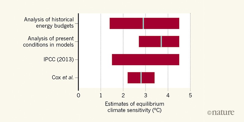
From Piers Forster:
“The best estimates of ECS that have been made by analysing Earth’s energy budget (the balance of the energy received by Earth from the Sun and the energy radiated back to space) are relatively low, at around 2 °C. But recent work is helping us to understand that ECS values inferred from energy-budget changes over the past century are probably low, and shows that a higher value is more applicable when projecting future change.”
All I can say to this is that nobody has helped me understand that “ECS values inferred from energy-budget changes over the past century are probably low.”
The key message of the paper is in the last sentence: “Our emergent constraint therefore greatly reduces the uncertainty in the ECS value of Earth’s climate, implying a less than 1 in 40 chance of ECS>4K, and renewing hope that we may yet be able to avoid global warming exceeding 2K.”
The paper reduces the upper field of ECS up to 4.5K and above.
SoD: I have a comment in moderation and I’m not aware of breaking the rules… 🙂
frankclimate,
That seems to happen at random sometimes. There are key words that can trigger moderation that are linked to a banned poster that has re-appeared as a sock puppet several times in the past. But sometimes it just happens. Probably the quickest way to get a post unmoderated is to email Science of Doom (all one word, lower case, using the domain gmail.com.
Frank, rescued from moderation – as always with your comments, no idea why WordPress had trapped it.
thanks SoD… as I’m not a native English speaker and I’m always cruitical to my own posts… sometimes I could break the rules without any knowledge of this.. happy to read that this was not the case 🙂
Thanks for the link to Cox et al. Seems a sensible approach to help constrain sensitivity, though the details of their methods matter. Too bad it is pay walled.
I’m not quite sure about the merit of the paper, I read it. The last sentence:”… and renewing hope that we may yet be able to avoid global warming exceeding 2K.” is some kind of odd because the 2K-target is mostly influenced by the TCR which was no issue of the paper. Silly…
Frank,
Well, TCR is likely somewhere between ~60% and ~75% of ECS (give or take a few %), with the higher percentage associated with relatively low ECS and the lower percentage associated with higher ECS. So a constraint on ECS, if accurate, should also help constrain TCR. 75% of 2C is 1.5C TCR; 60% of 3C is 1.8C.
Steve – per your “what an odd comment”
A 3 ECS model, like that used in Dessler et. al., would match natural variability well if Cox et. al is correct.
Yes frank, this paper seems to be yet another installment in the emergent constraint category. The emergent constraint is if I read correctly just short term temperature variability. The only problem here is that the result is contradicted by other emergent constraint papers as I recall several showed that ECS of 4+ was more likely.
Frankclimate: I haven’t had a chance to read Cox, but I have listened to a podcast interview he made before the release of this paper. The top and bottom bars are improved energy-balance methods, combining models and observations. That approach is attractive because it combines the strengths of each: the real-world with perfect physics but very limited observations and only a single realization; and the model-world with imperfect physics but perfect observations and multiple realizations.
I think I hold on to my nullhypothesis, that cloud feedback is zero.
CERES Edition 4 and the Cloud Radiative Effect
Willis Eschenbach. wattsupwiththat.com/2018/01/18
“First, note that the global average change of CRE with temperature is 0.0 W/m2 per degree C. This might explain why there is so much debate even as to the sign of the change in cloud radiative effect with increasing temperature.”
Analysis of CERES data mar -2000 to feb -2017.
Another paper from an author participating in the CFMIP:
Interactions between Hydrological Sensitivity, Radiative Cooling, Stability, and Low-Level Cloud Amount Feedback
A helpful explanation:
<a href="https://www.atmos.washington.edu/~robwood/topic_eis.htm"estimated inversion strength (EIS)
Using CERES data it seems to be a close connection between equatoric sea surface warming and evaporation. From Willis Eschenbach:
“By the time you get up to 28°C or 29°C, the evaporative cooling is increasing at a remarkable rate. In practice, this means that at ocean temperatures up near 30°C, any extra incoming solar energy merely increases evaporation, with only a minimal increase in the sea surface temperature. This keeps the average sea surface temperature under 30°C everywhere in the open ocean.”
This will show up in rainfall 8condensation) and water vapor transport (potential energy). This can explain the increase of cloud cover the last 100 years.
This post is deeply flawed. It assumes that the location where rain falls is the location where evaporative cooling occurred. The average water molecule in the tropics remains in the atmosphere for 5 days (total column water divided by precipitation rate) and for 9 days outside the tropics. Trade winds and extratropical winds transfer water vapor many thousands of kilometers from the point where evaporation occurs to the point where precipitation occurs, something Willis totally ignores
The truth is that the rate of evaporation is proportional to wind speed and undersaturation (1-relative humidity). Temperature plays no role in evaporation except by increasing undersaturation when temperature rises. See links below. (SSTs varies less than 1 degC between night and day. Willis’s thermostat hypothesis applies to tropical islands that warm rapidly during the day, not tropical oceans.)
https://www.gfdl.noaa.gov/blog_held/47-relative-humidity-over-the-oceans/
Relative humidity is anti-correlated with temperature in the tropics (higher temperature, more evaporation) but correlated elsewhere (higher temperature, less evaporation). Figure 4 of Pfahl, S., and N. Niedermann (2011), Daily covariations in near‐surface relative humidity and temperature over the
ocean, J. Geophys. Res., 116, D19104, doi:10.1029/2011JD015792.
Average wind speed:
https://www.climate-charts.com/World-Climate-Maps.html
Map of resulting latent heat flux. There is a generally a greater flux of latent heat where it is warmer, but the reasons are complicated.
http://climvis.org/anim/maps/global/lhtfl.html
From your reference. Held:
“However, the models do seem to take advantage of the simplest way of throttling back the evaporation — a small increase in RH.”
This could be a critical point. Perhaps the small increase in RH is to little to make a noticeable difference? There has to be a consequence of warming that the air flow is increasing. Then the moist air is transported away more effectively. And it will drag in more dry air. So it will be natural with some thermostat effect on a local bases. Perhaps with more latent heat to radiate away on global bases.
Frank wrote: “The truth is that the rate of evaporation is proportional to wind speed and undersaturation (1-relative humidity). Temperature plays no role in evaporation except by increasing undersaturation when temperature rises.”
The rate of evaporation does depend on wind speed (but not proportional, I think) and undersaturation. But it is also directly proportional to equilibrium vapor pressure. That depends strongly on temperature.
I agree that Willis’s interpretation of his plot seems deeply flawed. But it is still a fascinating plot.
Mike wrote: “The rate of evaporation does depend on wind speed (but not proportional, I think) and undersaturation. But it is also directly proportional to equilibrium vapor pressure. That depends strongly on temperature.”
Thanks for the reply. (I learn a lot from you. In this case, however, I think you are confusing saturation vapor pressure at EQUILIBRIUM – where no evaporation occurs unless temperature is changing – with the non-equilibrium situation that exists in the air over the ocean. There, the rate-limiting step in evaporation is the need to transfer water molecules vertically away from the surface, which is controlled by turbulent mixing of wind speed (until the wind is strong enough to produce a spray of water droplets). And the higher the relative humidity of the air over the ocean, the faster water molecules travel from the air to the ocean. Evaporation is the net flux of a water molecules moving in both directions.
Willis’ plot is fascinating. Earlier posts have caused me to research the geography of relative humidity, wind speed, and the resulting flux of latent heat. Only one of these maps displayed in my post above. I hoped to show all three.
The Western Pacific Warm Pool has weak winds and relative humidity that rises modestly with temperature, providing a flux of latent heat much smaller than predicted from rainfall.
NK quotes Held: “However, the models do seem to take advantage of the simplest way of throttling back the evaporation — a small increase in RH.”
Yes. This is because the overturning of the atmosphere – which is what controls relative humidity over the ocean – slows down in the models. Overturning is due to convection and precipitation – phenomena that are parameterized in models. This slowing is essential to matching the increased surface flux of latent with warming (W/m2/K) with the increase in radiative cooling to space with surface warming (W/m2/K). The later is climate sensitivity in units of K/(W/m2)). So this parameterized phenomena is as fundamental to climate sensitivity as WV, LR, and cloud feedbacks.
Along these lines, evaporation seems to be greater in the winter hemisphere, while precipitation is greater in the summer hemisphere ( suggesting transport ).
The effect of the windier winter hemisphere, with dry air masses pouring out over the oceans, does seem to trump the effects of temperature and insolation.
There is one fundamental issue I do not understand. Two quotes from the article:
“cooling from reflecting sunlight (albedo effect) of about 46W/m²”
“warming from the radiative effect of about 28W/m² – clouds absorb terrestrial radiation and reemit from near the top of the cloud where it is colder, this is like the “greenhouse” effect”
“If high clouds increase in altitude the radiation from these clouds to space is lower because the cloud tops are colder”
So we have reflections and emissions, and they go either upward (into space..) or downward. According to this, we would not at all have downward reflections of terrestrial IR. Upward IR emissions however .. well we have them, and then again not. When determining the net CF (cloud forcing), should we not take upward emissions into account (as cooling), rather than only accounting for the albedo effect? But then, if we do, how could we ever make sense of this model. Also the named albedo effect of 46W/m2 seems very low. As compared to this for instance..
https://www.weather.gov/jetstream/energy
Here it is 23% for the albedo effect and 9% for upward emissions (of 342W/m2 = 100%), which total 32% or 110W/m2. 110W/m2 upward radiation (reflection and emissions) vs. 46W/m2 is a big deal. That is next to the question if upward emissions do exist at all.
Furthermore I took a closer look on real life data from US weather stations. These data (2015-2017) include cloudiness (up to and altutide of 12.000ft only!) and temperature. The cloud condition would be broken in to five categories (CLR, FEW, SCT, BKN, OVC). The tropical sample showed this result:
There may be specific reasons, why low cloud OVCs show an eventuall drop in temperatures (rain, thunderstorms..). Yet, there seems to be basic correlation. The more clouds, the higher the temperatures. And this goes for low tropical clouds, which are meant to have to strongest negative net forcing.
IIRC, incomplete cloud cover can actually increase surface insolation. What’s lost to the occasional cloud covering the sun for a time may be more than made up for by scatter from clouds that don’t cast a shadow on a given location. But that’s all short term. The long term effect should still be more low clouds lowers the average temperature.
Leitwolf wrote: “So we have reflections and emissions, and they go either upward (into space..) or downward. According to this, we would not at all have downward reflections of terrestrial IR. Upward IR emissions however .. well we have them, and then again not.
From some perspectives, climate sensitivity is all about how fast TOA OLR and reflection of SWR (OSR) change with rising Ts. If OLR+OSR increases 1 W/m2 per degC rise in surface temperature, then the the 3.7 W/m2 imbalance created by doubling CO2 will be corrected by a warming of 3.7 K. If the increase is 2 W/m2/K, half as much warming will be needed. This is called the climate feedback parameter and is usually written with a negative sign for heat lost.
DLR and upward LWR absorbed by clouds don’t have any direct impact on OLR+OSR – they merely redistributes heat from within the climate system. They do change local temperature. However, if we specify a surface temperature and lapse rate, we have a simple model of the atmosphere that doesn’t require deeper analysis of internal heat transfer. So the main focus is on OLR and OSR.
Reflection of SWR is somewhat independent of temperature (except for clouds made of ice vs water droplets). Emission of OLR, of course, depends on temperature. The LWR photons that escape to space (the only ones that matter to climate sensitivity) through clear skies originate from the surface and all altitudes, but the average height is about 5 km. Those that come from the surface have a blackbody spectrum, while those that come from GHGs in the atmosphere do not. When clouds are present, this clear sky emission is replaced by blackbody radiation characteristic of the cloud top temperature, modified by the GHGs between the cloud top and space (where atmosphere is relatively dry and thin). So high cloud tops can emit much less OLR compared with clear skies negating the SWR they reflect, while low cloud tops emit almost as much OLR as clear skies (while reflecting a lot of SWR).
The Figure below shows that about half of OSR (100 W/m2) comes from clear skies (surface albedo and aerosols), while the other half comes from clouds, roughly consistent with SOD’s value of 46 W/m2. (I’m somewhat surprised at the even split.)
http://www.pnas.org/content/110/19/7568

The globally averaged, monthly mean TOA flux (Wm−2) of annually normalized, reflected solar radiation over all sky (A) and clear sky (B) and the difference between them (C) (i.e., solar CRF) are plotted against the global mean surface temperature (K) on the abscissa.
Thanks Frank
There are problems back and forth with all these arguments.
“DLR and upward LWR absorbed by clouds don’t have any direct impact on OLR+OSR – they merely redistributes heat from within the climate system”
That mechanism is nothing less than the GHE itself. If upward LWR and (re-emitted) DLR were merely a redistribution within the climate system, with a neutral role, than clouds could not serve as a “GHG”, nor could any other GHG.
Next we have the issue of the very low (cloud) albedo. If out OSR was indeed only 100W/m2, than the Earths albedo would be only 100/342 = 0.29. I would assume it to be rather 0.31, but who knows. What I subject to is an “island solution” where albedo all of a sudden drops to argue one specific point. We should be more consistent.
Also a mere 50W/m2 (or even less !?) for cloud albedo will not make a lot of sense. The cloud free albedo of Earth is indeed very low (much lower than that of the moon by comparison), I ran my own research on it. Ocean water is about 0.06, total clear sky albedo <0.1. Both true however for visible light only. So indeed clouds will provide more than 2/3s to the total albedo.
On the other side, if we assumed cloud albedo to amount to only 50W/m2 globally, with text book albedo for clouds ranging from 0.6 to 0.9, these figures will not add up. I mean even we took the low end of 0.6, it would mean a total average cloud cover of only (50/342)/0.6 = 24.4%. We have much higher figures than that throughout the literature.
Also we run into trouble with the suggested negative CF, which can only be attributed to cloud covers (clouds can not have any forcing with a clear sky obviously). A negative net forcing of -20W/m2 coming from just 24.4% cloud cover, would mean -20/0.244 = -82W/m2 with a solid overcast sky. Not quite realistic obviously.
I could go on like that for quite a while. The point is, these figures are neither true, nor consistent with other representations of the consensus model. Also it will not giive any answer to why ignore OLR of clouds when determining their net CF.
So there is plenty of cherry picking and data bending. The problem itself, which I described above, is not even tackled by it. We have upward and downward radiation by clouds. Upward radiation will be around 110W/m2, downward radiation is in question (and part of the GHE!), just as the net CF.
So the basic problem is, how to get from 110W/m2 upward, to a small downward radiation, while not getting high on a net negative CF. Mathematically that seems impossible. Let us put into a simple formula, with DR – UR = NF. (DR = down radiation, UR = up radiation, NF net forcing).
30 – 110 = -20 ,, will not work obviously.
I do understand how flip-floping and manufacturing data may be the only "solution", but I will not buy it.
Leitwolf,
You’ve left out an important contribution to clear sky albedo, snow and ice which have a high reflectivity. In your diagram, 7% of incoming solar radiation is reflected back to space by the surface. That would seem to imply an albedo for the surface of 0.07. However, given that ~60% of the surface is covered by clouds on average, that means 7% of the radiation is reflected by 40% of the surface for an albedo of 0.07/0.4 = 0.175. Take a look at a plot of albedo vs. sine(latitude) (to correct for area): https://i.imgur.com/MaZopg6.png
Note the increase in albedo at high latitudes. That’s snow and ice.
Leitwolf,
According to Wikipedia:
https://en.wikipedia.org/wiki/Albedo
So minimum cloud albedo is a lot lower than 0.6. I do question the relative sizes of the solar radiation absorbed by atmosphere and absorbed by clouds, though. Water droplets absorb strongly in the near IR and a substantial fraction of solar energy is in the near IR.
Thanks Payne (is that a first name?)
Of course snow and ice will increase albedo, but both will be located in places where there is only little sun shine. In fact the lack of solar input is the reason why there is ice and snow in the first place. So even while they may cover like 4% of the surface, they will only receive like 1-1.5% of solar radiation. Ultimately they will increase total albedo by maybe ~1%. It is a factor, but not a very important one.
If 60% of the surface was covered by clouds (again, I am willing to see different perspectives, but they should be consistent in the end), and their contribution to albedo was only 0.14, like suggested by Franks post, these clouds would end up being not quite reflective. 0.14/0.6 = 0.23. Then these clouds could only relfect 23% of sun light hitting them, which makes little sense.
Ultimately it is about the definition of a “cloud”. If a cloud can have an albedo of zero, it is no more a cloud, as it is not even visible. If we are talking about thin, transparent clouds, I from my perspective would only count them to the degree of their opaqueness. Otherwise we put very opposite things all into one bag, without differentiating.
In the picture below, is that a 100% cloud cover with 95% transparency, or a 5% cloud cover, with a 100% opaqueness? Is the glas half full, or half empty..?
Leitwolf wrote: “Next we have the issue of the very low (cloud) albedo. If out OSR was indeed only 100W/m2, than the Earths albedo would be only 100/342 = 0.29. I would assume it to be rather 0.31, but who knows.”
I think the albedo has been revised down to 0.29 from the value of 0.31 that I learned as a boy.
Leitwolf wrote: “Also a mere 50W/m2 (or even less !?) for cloud albedo will not make a lot of sense. The cloud free albedo of Earth is indeed very low (much lower than that of the moon by comparison), I ran my own research on it. Ocean water is about 0.06, total clear sky albedo <0.1. Both true however for visible light only. So indeed clouds will provide more than 2/3s to the total albedo."
You have overlooked an important factor: clear sky Rayleigh scattering from the atmosphere (the same mechanism that causes the sky to be blue). Stephens et al [2012] (I'll provide full reference if you don't mind a paywall) gives the following numbers:
48 W/m^2 reflection from clouds
27 W/m^2 reflection from clear sky
23 W/m^2 reflected from surface
100 W/m^2 total reflected
They don't quite add up, but the uncertainties are all in the range 2 to 5 W/m^2. The total seems to be the best known number of the lot.
Leitwolf,
Payne is my surname. My given name is DeWitt. No offense taken since both my surname and given name are used by others as either, for example the late golfer Payne Stewart or the actress Joyce DeWitt.
You’re way underestimating the surface area where snow and ice are significant contributors to albedo. About 60% of the Earth’s surface has an average albedo of less than 0.3. Clouds alone won’t get you an average albedo above 0.3. Also, while the poles are dark for half the year, at peak summer insolation, they receive more energy/day than low latitudes because the sun is above the horizon all day.
Hi Mike!
I definitely do not believe these figures, and here is the (obvious) reason why:
When I was talking about clear sky albedo, that already includes light reflected by the atmosphere. So the brightness of clear sky areas are surface albedo + “atmosphere albedo”, if you will. And that sum is just so much darker than the surface of the moon, that both together are definitely <0.1. The moons albedo is 0.13 at best btw.
The picture above was taken from NASAs DSCOVR satellite, and you may want to analyze it yourself. It may help converting it to a black/white picture and cutting out parts, to make direct comparisons. Also there are tools that will tell you the exact color of a single pixel. Btw. you can easily find more of these pictures online.
My conclusion is this: above the ocean (clear sky) albedo is roughly half of that of the moon, and over land it is rougly the same. Again, this is true for visible light. Things might be somewhat different for UV and IR light, which I can not see and henceforth not judge. But visible light is already accounting for about 50% of total solar radiation, and short wave IR will not behave very differently.
Also this judgement is completely in line with the figures presented throughout literature. It was never at doubt, that clouds make up for over 2/3s of the total albedo.
As I stated before however, this will necessarily lead to an open dissent within the GH-model with regard to the accounting of cloud forcing. And to me it looks like, as if there figures were just manufactured to deal with this dissent, rather than giving correct assessments. Btw. I have drawn a simple chart to illustrate the contradicting versions of CF (the right side is based on the 1990 IPCC report, according to which it were 44W/m2 albedo effect, and 31W/m2 down-forcing by emissions)..
Leitwolf. I wonder if this is your understanding of the greenhouse effect?
“However there is one thing which I am completely certain of. Even in the absence of a GHE, given that sunlight is also warming the atmosphere, not just the surface, we would have “back radiation”. So you must not consider “back radiation” as evidence for a GHE. That would be a logical mistake.”
Leitwolf: Glad to be of some help.
Although you are entitled to your own opinion, I don’t think it makes much sense to debate the numbers being reported by CERES and incorporated into energy flux diagrams.
One of the K&T energy balance diagrams says that 79 W/m2 of SWR is reflected by clouds and ATMOSPHERE (Mike’s scattering) and 23 W/m2 by the surface. So the clear skies reflection of about 50 W/m2 could be about half from the surface and about half from scattering by the atmosphere. (These are very similar to the numbers Mike cited.) The reason that reflection of SWR increases during winter in the NH is due to land covered with seasonal snow (which the SH has very little).
I must admit to being confused with some of the terminology: cloud forcing (CF), cloud radiative effect (CRE), and cloud radiative forcing (CRF) – which may all be the difference between all skies and clear skies, and feedbacks in any of these (dCRE/dT). Then we the cloud fraction and feedback in it. If clear skies reflect an average of 50 W/m2 and all skies (which are 2/3rds cloudy) reflection 100 W/m2, then cloudy skies must reflect 125 W/m2. There is also a cloud albedo. And we have SWR and LWR components of some of these.
Click to access acp-11-7155-2011.pdf
I prefer to think of the GHE as 390-240 = 150 W/m2. It is a consequence of the temperature gradient in the atmosphere and therefore of all radiative and convective fluxes. (An isothermal atmosphere has no GHE.)
Btw. I find this video quite fascinating, and it seems a bit odd we don’t have more of that kind. Are these clouds emitting or reflecting IR?
https://www.videoblocks.com/video/urban-heat-islands—infrared-thermal-video-warming-city-time-lapse-hxw3kmvt-eivokp2m7
@Frank
The debate should not be so much on (CERES) data (which are a black box after all), but on their interpretation.
With that link, and I do not think I quite understand it, is Fig.11 suggesting an average (global) cloud albedo of about 0.26? That would be 0.26 * 342 = 89W/m2 ?? I mean they obviously multiply cloud fraction with cloud albedo, and logically that is the indicated result.
FWIW, Nic Lewis continued his comment at WUWT with the following information that answered a number of my questions.
“In CMIP5 models that include indirect aerosol forcing (the effect of aerosols on clouds; ACI), the average total aerosol forcing change over 1850-2000 is about -1 W/m^2, maybe a bit more. In some models is approaches -1.5 W/m^2. Direct aerosol forcing (the effect of aerosol-radiation interations; ARI), which is all that a few models include, is typically -0.35 to -0.4 W/m^2.
So indirect aerosol forcing averages approaching -0.7 W/m^2. Part of that is the cloud albedo (1st indirect) or Twomey effect; aerosols making clouds brighter, due to seeding more but smaller cloud droplets. But the cloud lifetime (2nd indirect) or Albrecht effect is probably somewhat more important in models. The idea is that clouds with smaller droplets have more water (a larger Liquid Water Path) and last longer. Obserations do not support this effect. This study corroborates, on a global scale, another recent study (Siefert et al 2015, DOI: 10.1002/2015MS000489) that studied particular regions and found the cloud lifetime effect to produce a positive forcing.
The implication is that the 2nd indirect aerosol effect may well pretty much cancel out the 1st effect. That would mean most CMIP5 models have aerosol forcing that is 0.5 to 0.75 W/m^2 too negative. Removing that excess aerosol forcign will make the models’ historical simulations warm too fast over 1850-2005. As the new studies say, GCMs “tend to be optimised to adjust the magnitude of the aerosol indirect effect so that the models reproduce historical climate changes”.”
These developments aren’t surprising given Section 7.4.3 orAR5 WG1, which prefers to think of the combined Twomey and Albrecht effects as a single phenomena that affects clouds warm enough to be all liquid:
“The adjustments giving rise to ERFaci are multi-faceted and are associated with both albedo and so-called ‘lifetime’ effects (Figure 7.3). However, this old nomenclature is misleading because it assumes a relationship between cloud lifetime and cloud amount or water content. Moreover, the effect of the aerosol on cloud amount may have nothing to do with cloud lifetime per se (e.g., Pincus and Baker, 1994).
The traditional view (Albrecht, 1989; Liou and Ou, 1989) has been that adjustment effects associated with aerosol–cloud–precipitation interactions will add to the initial albedo increase by increasing cloud amount. The chain of reasoning involves three steps: that droplet concentrations depend on the number of available CCN; that precipitation development is regulated by the droplet concentration; and that the development of precipitation reduces cloud amount (Stevens and Feingold, 2009). Of the three steps, the first has ample support in both observations and theory (Section 7.4.2.2). More problematic are the last two links in the chain of reasoning. Although increased droplet concentrations inhibit the initial development of precipitation (see Section 7.4.3.2.1), it is not clear that such an effect is sustained in an evolving cloud field. In the trade-cumulus regime, some modeling studies suggest the opposite, with increased aerosol concentrations actually promoting the development of deeper clouds and invigorating precipitation (Stevens and Seifert, 2008; see discussion of similar responses in deep convective clouds in Section 7.6.4). Others have shown alternating cycles of larger and smaller cloud water in both aerosol-perturbed stratocumulus (Sandu et al., 2008) and trade cumulus (Lee et al., 2012), pointing to the important role of environmental adjustment. There exists limited unambiguous observational evidence (exceptions to be given below) to support the original hypothesised cloud-amount effects, which are often assumed to hold universally and have dominated GCM parameterization of aerosol–cloud interactions. GCMs lack the more nuanced responses suggested by recent work, which influences their ERFaci estimates.
Maybe of interest in relation to ERF Aerosols: A recent paper https://www.nature.com/articles/s41467-018-03379-6 finds that the ERFaci ( aerosol-cloud- interaction) is near zero or even slightly positive. This would reduce the Aerosol Forcing tot. about 30…50% with huge impacts on the sensivity ( decreasing) of the real world vs. CO2. Any thoughts?
The aerosol indirect effect always was something of a fudge factor. I remember a post on Pielke, Sr’s blog years ago that was of the opinion that it was a lot smaller, likely zero, than what was assumed in the models. I never could find it again, though.
I thought the aerosol indirect effect was based on cloud microphysics and the observation of ship tracks (https://en.wikipedia.org/wiki/File:ShipTracks.jpg). Qualitatively it seems quite sound. More particles and/or larger particles should lead to more cloud droplets. For a given amount of liquid water, that means more surface area and more reflection. The amount of liquid water, which governs IR absorption, is unaffected since that is controlled by thermodynamics, not kinetics. I think the effect is expected to be strongest in marine stratus clouds, which is where ship tracks are observed.
This new study:Aerosol effects on cloud water amounts were successfully simulated by a global cloud-system resolving model
Yousuke Sato, Daisuke Goto, Takuro Michibata, Kentaroh Suzuki, Toshihiko Takemura, Hirofumi Tomita & Teruyuki Nakajima
It is about how condensation and evaporation in clouds is affected by the size of cloud particles, and the size of cloud particles is affected by aerosols. Models have not been able to simulate this in a good way earlier.
From the peer rewiev file: “As we shown in Fig. 2b, the condensation tendency increased in the lower part of cloud (~ 500m from the cloud bottom). In contrast, the evaporation tendency increased in the upper part of cloud as shown in Fig. 2c. The responses of the processes are both originated from the reduction of cloud particle size with the increase of aerosols. However, the reduction of cloud particles resulted in different story depending on the moisture of ambient air. In the lower part of cloud, the ambient air was moist (Fig. 2d) and the condensation tended to be promoted, when the cloud particle size is reduced by the increase of aerosol. On the other hand, the dry air in the upper part of clouds (Fig. 2d) promoted the evaporation process when the cloud particle size is reduced by the increase of aerosol amount. The promotion of evaporation in the upper part and that of condensation in the lower part of cloud occurred regardless of the stability. “
From Nic Lewis at WUWT:
“This is an important paper. It shows that when a much higher resolution global climate model that is able to resolve clouds, including as to their depth, is used the sign of the aerosol “cloud lifetime effect” radiative forcing is positive. By contrast, in all but a few models that forcing is significantly negative, and is one of the main reasons why current climate models match observed historical warming despite their generally high (transient) sensitivity.”
What is interesting is the leap. There is obviously another direction this can go.
FWIW, Nic Lewis continued his comment at WUWT with the following information that answered a number of my questions.
“In CMIP5 models that include indirect aerosol forcing (the effect of aerosols on clouds; ACI), the average total aerosol forcing change over 1850-2000 is about -1 W/m^2, maybe a bit more. In some models is approaches -1.5 W/m^2. Direct aerosol forcing (the effect of aerosol-radiation interations; ARI), which is all that a few models include, is typically -0.35 to -0.4 W/m^2.
So indirect aerosol forcing averages approaching -0.7 W/m^2. Part of that is the cloud albedo (1st indirect) or Twomey effect; aerosols making clouds brighter, due to seeding more but smaller cloud droplets. But the cloud lifetime (2nd indirect) or Albrecht effect is probably somewhat more important in models. The idea is that clouds with smaller droplets have more water (a larger Liquid Water Path) and last longer. Obserations do not support this effect. This study corroborates, on a global scale, another recent study (Siefert et al 2015, DOI: 10.1002/2015MS000489) that studied particular regions and found the cloud lifetime effect to produce a positive forcing.
The implication is that the 2nd indirect aerosol effect may well pretty much cancel out the 1st effect. That would mean most CMIP5 models have aerosol forcing that is 0.5 to 0.75 W/m^2 too negative. Removing that excess aerosol forcign will make the models’ historical simulations warm too fast over 1850-2005. As the new studies say, GCMs “tend to be optimised to adjust the magnitude of the aerosol indirect effect so that the models reproduce historical climate changes”.”
These developments aren’t surprising given Section 7.4.3 orAR5 WG1, which prefers to think of the combined Twomey and Albrecht effects as a single phenomena that affects clouds warm enough to be all liquid:
“The adjustments giving rise to ERFaci are multi-faceted and are associated with both albedo and so-called ‘lifetime’ effects (Figure 7.3). However, this old nomenclature is misleading because it assumes a relationship between cloud lifetime and cloud amount or water content. Moreover, the effect of the aerosol on cloud amount may have nothing to do with cloud lifetime per se (e.g., Pincus and Baker, 1994).
The traditional view (Albrecht, 1989; Liou and Ou, 1989) has been that adjustment effects associated with aerosol–cloud–precipitation interactions will add to the initial albedo increase by increasing cloud amount. The chain of reasoning involves three steps: that droplet concentrations depend on the number of available CCN; that precipitation development is regulated by the droplet concentration; and that the development of precipitation reduces cloud amount (Stevens and Feingold, 2009). Of the three steps, the first has ample support in both observations and theory (Section 7.4.2.2). More problematic are the last two links in the chain of reasoning. Although increased droplet concentrations inhibit the initial development of precipitation (see Section 7.4.3.2.1), it is not clear that such an effect is sustained in an evolving cloud field. In the trade-cumulus regime, some modeling studies suggest the opposite, with increased aerosol concentrations actually promoting the development of deeper clouds and invigorating precipitation (Stevens and Seifert, 2008; see discussion of similar responses in deep convective clouds in Section 7.6.4). Others have shown alternating cycles of larger and smaller cloud water in both aerosol-perturbed stratocumulus (Sandu et al., 2008) and trade cumulus (Lee et al., 2012), pointing to the important role of environmental adjustment. There exists limited unambiguous observational evidence (exceptions to be given below) to support the original hypothesised cloud-amount effects, which are often assumed to hold universally and have dominated GCM parameterization of aerosol–cloud interactions. GCMs lack the more nuanced responses suggested by recent work, which influences their ERFaci estimates.
Frank, quoting Nic Lewis: “Part of that is the cloud albedo (1st indirect) or Twomey effect; aerosols making clouds brighter, due to seeding more but smaller cloud droplets. But the cloud lifetime (2nd indirect) or Albrecht effect is probably somewhat more important in models. … The implication is that the 2nd indirect aerosol effect may well pretty much cancel out the 1st effect.”
Thanks, to both Frank and Nic. I had forgotten about the Albrecht effect, probably because it has always been speculative as to sign. So I never realized that it is so important in models. I wouldn’t guess that based on the text in AR5; at least, not without impugning motives. I had assumed that uncertainty in the indirect effect was due to uncertainty in the Twomey effect.
I am not a scientist nor a chemist but am curious as to the chemical interaction between methane and water vapour clouds. We see more articles lately about the possibility of 1+ gigaton sudden methane emissions from the warming Arctic region. My question is whether the atmospheric chemical reaction of such large methane outbursts will lead to extensive water vapour clouds (normally restricted to the troposphere/tropopause) forming in the stratosphere. If so would they significantly reflect away solar radiation, and if so for how long and with what other effects?
Mike: Methane doesn’t form clouds in our atmosphere because its boiling point is too low (-164 degC, 109 K, about 75 degC below the coldest place on the planet). However, methane and water can freeze together (co-crystallize) to make a solid (“ice” or clathrate) that contains 5 methane molecules for every 23 water molecules. The stability of the clathrate depends on both temperature and pressure. These clathrates has been found in oceans and permafrost.
There is fear that climate change will release large amount of methane from clathrates. As with CO2, the amount of methane in the atmosphere increases about 50% during interglacials (5 degC of warming). However, during the industrial era methane has already more than doubled, so potential danger from methane released by warming alone APPEARS modest compared with other changes. However historical change has been much slower than we may experience in the next century. Fortunately, the half-life of methane in the atmosphere is only 10 years.
I think Mike was referring to the production of stratospheric water vapor by methane oxidation. That would not form clouds, but would increase the size of stratospheric particles and increase solar reflection. I would think the effect would be very much smaller than what occurs after a big volcanic eruption, but it would last longer.
ECS is just a modeling benchmark that can never exist in the real world. Why then the seeming obsession with it? Maybe focus more on the far more important model failure (ESMs in this case) re warm paleoclimates like the mid-Pliocene? Beyond that, there are Earth system feedbacks that don’t exist at equilibrium (the real-world one related to Earth system sensitivity). Could an unnaturally rapid warming pace increase their magnitude greatly relative to the past? Probably.
Background: Hansen et al. “Target CO2” paper (10th anniversary!), also this current article aimed at a more general audience.
Note for anyone who has issues with paper access: Sci-Hub.
Corrected first link.
Steve: I like to focus on the reciprocal of ECS – the climate feedback parameter usually reported in W/m2/K. That quantity feels more “real” than a “modeling parameter”. It is a measure of how our planet responds to ANY change in average Ts with a change in radiative cooling to space.
ECS is a temperature change that is approached in about a century in response to a doubling of CO2. The climate feedback parameter describes what happens to radiative cooling to space after a change in Ts and is – for the most part – complete within a month or two after a change in surface temperature. The response to the seasonal 3.5 K increase in GMST (produced by hemispheric changes in irradiation and the lower heat capacity of the NH) is very linear with a slope of 2.2 W/m2/K from both clear and all skies. AOGCMs produce the same result from clear skies (where only WV, LR and Planck feedbacks operate), but produce too positive a cloud LWR feedback from cloudy skies. (If this were all that were important, ECS would be 1.7 K and the debate would be over.)
Unfortunately, the seasonal change in reflection of SWR is not a linear function of temperature, so we shouldn’t use it to calculate feedbacks (dOSR/dTs). Changes in SWR reflected through clear skies report changing surface albedo arising from seasonal snow cover and sea ice. The response of these phenomena lags months behind changes in surface temperature, but mostly don’t require years. And there are huge hemispheric differences in seasonal snow cover and sea ice caused by geography rather than Ts. And it turns out that seasonal changes in the reflection of SWR by clouds does not depend linearly on Ts either. AOGCMs disagree with each other and observations about how reflection of SWR should change seasonally.
The climate feedback parameter is also useful in thinking about the time scale of the radiative response of our planet to changes in Ts. LWR and clouds respond in a month or two, seasonal snow cover in a few months, sea ice in months to a few years, surface vegetation in years to decades?, ice caps and ocean uptake of CO2 respond in centuries to millennia. These are all responses to changing Ts – feedbacks. The concepts of ECS and ESS place an arbitrary dividing line across these time scales – the amount of time it takes for the radiative imbalance at the TOA to approach zero in a 2X or 4X experiment with a climate model. Those feedbacks realized in such experiments become part of ECS. IIRC those that don’t are treated as forcing in ESS.
Steve: Advising society about what it needs to do today about GHGs and climate change takes a great deal of hubris. Imagine the government regulating or taxing our economy a century ago with the intention of trying to making the world a better place today. (An effort bigger than the space program or the Manhattan project persisting indefinitely.) How wisely would our predecessors have used that money (or the equivalent in lost economic growth through regulation)? When you look at current efforts to decarbonize the world’s economy, do you see any reason to think that our descendants a century from now will view as being any more brilliant that you perceive your predecessors a century ago?
Hansen’s Target CO2 paper asks us to worry about what will happen in millennia, not merely centuries. That world will be unimaginably different, even without GHG-mediated climate change. The absence of an ice-cap on Greenland and a diminishing ice cap in Antarctica will probably rank far down list of important changes.
From a comment I made to a Hansen et al paleoclimate study: “The Holocene and Eemian temperatures deserves a serious investigation. And not just throwing out some numbers that suits a political agenda. The temperatures say something about climate sensitivity and natural variation. If the Eemian temperatures in average were over one degree warmer than today, and CO2 consentration was around 270 ppm, there are some interesting questions about how this can happen.”
I am afraid there is much cherrypicking of data to make impact.
“Plotting GHG forcing [7] from ice core data [18] against temperature shows that global climate sensitivity including the slow surface albedo feedback is 1.5°C per W/m2 or 6°C for doubled CO2 (Fig. 2), twice as large as the Charney fast-feedback sensitivity”
I can understand that it can make you all scared, James Hansen, Makiko Sato, Pushker Kharecha, David Beerling, Robert Berner, Valerie Masson-Delmotte, Mark Pagani, Maureen Raymo, Dana L. Royer and James C. Zachos,
Activist fingerprint, from Hansen and friends: “Our estimated history of CO2 through the Cenozoic Era provides a sobering perspective for assessing an appropriate target for future CO2 levels. A CO2 amount of order 450 ppm or larger, if long maintained, would push Earth toward the ice-free state. Although ocean and ice sheet inertia limit the rate of climate change, such a CO2 level likely would cause the passing of climate tipping points and initiate dynamic responses that could be out of humanity’s control. “
Reblogged this on Climate- Science.
What happened to the positive longwave cloud feedback?
According to Dessler et.al (2010) most of the global warming came from this longwave component, and Zelinka et.al followed this up.
And we learn that changing longwave radiation at TOA comes from changing clouds, not from clear-sky (Wing et.al, 2017).
And then we learn that longwave radiation at TOA has increased over the years from 1985 to 2017. (DeWitte et al, 2018) ” From the joint analysis of the HIRS OLR and the NASA GISS global surface temperature anomaly, we derive an empirical estimate of the longwave climate feedback parameter dOLT/dT of 2.93 +/− 0.3 W/m2K 1 σ uncertainty interval.”
I think this is quite confusing
Dessler 2010: «The observations show that 60 to 80% of the total cloud feedback comes from a positive long-wave feedback, with the rest coming from a weaker and highly uncertain positive short-wave feedback.»
Zelinka and Hartmann, 2010: Why is longwave cloud feedback positive? «Here it is shown that this robust positive longwave cloud feedback is caused in large part by the tendency for tropical high clouds to rise in such a way as to remain at nearly the same temperature as the climate warms. Furthermore, it is shown that such a cloud response to a warming climate is consistent with well-known physics, specifically the requirement that, in equilibrium, tropospheric heating by convection can only be large in the altitude range where radiative cooling is efficient, following the fixed anvil temperature hypothesis of Hartmann and Larson (2002).»
In a comment at SoD Dessler holds firm to this hypothesis (January 3. 2018): «The strength of the greenhouse effect is determined by the temperature difference between the radiator and the surface. As the difference increases, the effectiveness of the radiator at trapping heat increases. The FAT = fixed anvil temperature hypothesis says that high clouds won’t change temperature as the surface warms, meaning that the temperature difference between the surface and clouds increases. This is therefore a positive feedback.»
So the conclusion is that anvil clouds rule the climate. The positive longwave cloud feedback is affirmed. What happens to other kind of clouds is not so important. It seems that this was a widespread understanding. But not the only way to see how the Earth warms.
I think Trenberth and Fasullo came along with a groundbreaking view on climate change in 2009, looking at clouds from another side, in the paper: Global warming due to increasing absorbed solar radiation: «Global climate models used in the Intergovernmental Panel on Climate Change (IPCC) Fourth Assessment Report (AR4) are examined for the top‐of‐atmosphere radiation changes as carbon dioxide and other greenhouse gases build up from 1950 to 2100. There is an increase in net radiation absorbed, but not in ways commonly assumed. While there is a large increase in the greenhouse effect from increasing greenhouse gases and water vapor (as a feedback), this is offset to a large degree by a decreasing greenhouse effect from reducing cloud cover and increasing radiative emissions from higher temperatures. Instead the main warming from an energy budget standpoint comes from increases in absorbed solar radiation that stem directly from the decreasing cloud amounts. Climate model changes from 1950 to 2100 in energy‐related quantities provide a new perspective on issues important for climate change, and highlight the role of changing clouds that lead to an opening of an aperture for solar radiation. In contrast the conventional wisdom is that longwave (LW) radiation anomalies dominate the planetary imbalance and warming is from a “blanketing” effect.»
What was it about cloud longwave feedback?
Perhaps we could ask a winner of Nobel Prize for Physics 2021, Suykuro Manabe.
Some answers came in his 2001 paper: Influence of cloud feedback on annual variation of global mean surface temperature. Yoko Tsushima and Syukuro Manabe.
“Abstract. The goal of this study is to estimate the cloud radiative feedback effect on the annual variation of the global mean surface temperature using radiative flux data from the Earth Radiation Budget Experiment. We found that the influence of the cloud feedback upon the change of the global mean surface temperature is quite small, though the increase of the temperature is as much as 3.3 K from January to July. On a global scale, we found no significant relationship between either solar reflectivity of clouds or effective cloud top height and the annual cycle of surface temperature. The same analysis was repeated using the output from three general circulation models, which explicitly predict microphysical properties of cloud cover. On a global scale, both solar cloud reflectivity and cloud top height increase significantly with the increase of surface temperature, in contrast to the observation. The comparative analysis conducted here could be used as an effective test for evaluating the cloud feedback process of a model.”
But this was a long time ago. So the same authors did the same analysis 12 years later, with new data. Yoko Tsushima and Syukuro Manabe, 2013: Assessment of radiative feedback in climate models using satellite observations of annual flux variation.
And they came to the same conclusions.
“In the climate system, two types of radiative feedback are in operation. The feedback of the first kind involves the radiative damping of the vertically uniform temperature perturbation of the troposphere and Earth’s surface that approximately follows the Stefan–Boltzmann law of blackbody radiation. The second kind involves the change in the vertical lapse rate of temperature, water vapor, and clouds in the troposphere and albedo of the Earth’s surface. Using satellite observations of the annual variation of the outgoing flux of longwave radiation and that of reflected solar radiation at the top of the atmosphere, this study estimates the so-called “gain factor,” which characterizes the strength of radiative feedback of the second kind that operates on the annually varying, global-scale perturbation of temperature at the Earth’s surface. The gain factor is computed not only for all sky but also for clear sky. The gain factor of so-called “cloud radiative forcing” is then computed as the difference between the two.”
“The gain factor of the longwave feedback for all sky obtained here is 0.28 and is similar to 0.32 (i.e., that of clear-sky feedback), yielding −0.04 as the gain factor of longwave CRF. The result presented here suggests that clouds have relatively small effect upon the longwave feedback that operates on the annual variation. This is in agreement with the results obtained from the other two sets of data obtained from satellite observation used here.”
What is this? A negative cloud longwave feedback. And this is in contrast to cloud feedback from climate models which is positive.
ZOMG, Lindzen was right all along and the planet is cooling!
Manabe: “The result presented here suggests that clouds have relatively small effect upon the longwave feedback that operates on the annual variation”.
“The comparative analysis conducted here could be used as an effective test for evaluating the cloud feedback process of a model.”
And the result suggest that climate models are systematically biased, according to Manabe.
And the systematic biases of models are well known to climate scientists. But this longwave cloud bias is one of the central issues of how we can misunderstand global warming.
Trenberth is probably right when he says that it is the thinning of clouds that has given the global warming now.
Frank has a comment on Manabe earlier in this discussion. Desember, 30,2017.
NK: I’ve brought up Tsushima and Manabe PNAS (2013) about easily measured feedbacks to seasonal warming many times. At least one of SOD’s posts deals with an early study including Ramanathan. There are caveats that should be mentioned:
1) The feedbacks to seasonal warming are not the same as feedbacks to global warming. Seasonal changes involve large changes in polar and temperate zones and almost no change in equatorial regions. So it over-emphasizes feedbacks in non-equatorial regions. Seasonal warming is the net result of warming in the NH (50% land, lower heat capacity) and cooling in the SH (10% land, higher heat capacity). Since there is a large change in seasonal snow cover in the NH almost none in the SH, SWR feedbacks through clear skies are fairly irrelevant to surface albedo feedbacks to global warming.
2) The LWR response to seasonal warming from both clear and all skies is highly linear and shows negligible lag. The negative feedback from all skies and clear skies similar (about -2.2 W/m2 = -3.3 W/m2 Planck feedback + +1.1 W/m2 WV+LR feedback), so cloud LWR feedback is slightly positive but indistinguishable from zero. The SWR response to seasonal warming is not highly linear and suggests that at least part of the response is lagged. Lindzen and Spenser independently find that SWR responses to warming (not explicitly seasonal) fit best with a three-month lag.
3) Tsushima and Manabe say: “One can argue whether the strength of the feedback inferred from the annual variation is relevant to global warming. Nevertheless, it can provide a powerful constraint against which every climate model should be validated.”
There is a new article by Hans-Rolf Dübal and Fritz Vahrenholt, In the journal Atmosphere, September 2021: Radiative Energy Flux Variation from 2001–2020. Presented in Climate etc. Oktober 2021.
With the summary: “Radiative energy flux data, downloaded from CERES, are evaluated with respect to their variations from 2001 to 2020. We found the declining outgoing shortwave radiation to be the most important contributor for a positive TOA (top of the atmosphere) net flux of 0.8 W/m2 in this time frame. We compare clear sky with cloudy areas and find that changes in the cloud structure should be the root cause for the shortwave trend. The radiative flux data are compared with ocean heat content data and analyzed in the context of a longer-term climate system enthalpy estimation going back to the year 1750. We also report differences in the trends for the Northern and Southern hemisphere. The radiative data indicate more variability in the North and higher stability in the South. The drop of cloudiness around the millennium by about 1.5% has certainly fostered the positive net radiative flux. The declining TOA SW (out) is the major heating cause (+1.42 W/m2 from 2001 to 2020). It is almost compensated by the growing chilling TOA LW (out) (−1.1 W/m2). This leads together with a reduced incoming solar of −0.17 W/m2 to a small growth of imbalance of 0.15 W/m2.”
The Dübal and Vahrenholt paper, Radiative Energy Flux Variation from 2001–2020, have got some attention. And for good reason. It is an important discussion. But there are some problems with some of the claims that are made.
«Radiative energy flux data, downloaded from CERES, are evaluated with respect to their variations from 2001 to 2020. We found the declining outgoing shortwave radiation to be the most important contributor for a positive TOA (top of the atmosphere) net flux of 0.8 W/m2 in this time frame.»
According to the CERES data they present (TOA all sky), the trend is LW out 0,28 W/m2/decade (cooling), SW out -0,70 (warming), and solar reduction 0,03 (cooling), wich gives a TOA warming trend of 0,39 W/m2/dec. So far so good. And in good agreement with Loeb et al 2021. EBAF Trends (03/2000-02/2021) 0.37 + 0.15 Wm-2 per decade.
«The declining TOA SW (out) is the major heating cause (+1.42 W/m2 from 2001 to 2020).»
Trend SW out all sky -0,70 W/m2/dec withsolar reduction included (0,70 W/m2/dec TOA warming). Gives 1,40 W/m2 over 20 years. This major heating is composed of SW clear sky heating trend of -0,37 W/m2/dec and a SW cloudy sky heating trend of -0,78 W/m2/dec. In the TOA radiation energy bridge-chart (figure 14) this is shown as SW clear sky increase of 0,15 W/m2 and SW cloudy areas increase of 1,27 W/m2. And the solar change impact is -0,17 W/m2 for 20 years. A great difference between trend and energy bridge-chart.
Loeb et al has a SW TOA heating of 0,63W/m2/dec through albedo change, with clouds increasing absorbed SW Flux 0,44W/m2/dec and surface increased absorption 0,19W/m2/dec. In good agreement with Dübal and Vahrenholt. EBAF Trends (03/2000-02/2021) 0.68 + 0.12 Wm-2 per decade.
«It is almost compensated by the growing chilling TOA LW (out) (−1.1 W/m2).»
But as we have seen, the trend is only 0,28 W/m2/dec. This is composed of LW TOA flux clear sky 0,04W/m2/dec and LW cloudy sky 0,35 W/m2/dec. How can they claim so big «chilling» longwave cooling? It looks like they use the startpoint and endpoint of a graph, and that the «chilling» cooling at TOA was for the year 2020 relative to 2001. In the TOA radiation energy bridge-chart (figure 14) this is shown as LW clear sky increase of 0,46 W/m2 and LW cloudy areas increase of 0,64 W/m2. I think what is presented in the bridge-charts is close to cherrypicking.
Loeb et al EBAF Trends (03/2000-02/2021) -0.31 + 0.12 Wm-2 per decade
The Dübal and Vahrenholt calculations for cloudy areas are clearly showing how clouds are the greatest component of global warming.
Correction: the EBAF trends from Loeb et al shall have uncertainty, +- instead of only +.
From Loeb et al 2021 we learn that there is a longwave cloud cooling. It is -0,15 W/m2 pr decade. From: Satellite and Ocean Data Reveal Marked Increase in Earth’s Heating Rate. This agree with many other scientists, and measured radiation at Top Of Atmosphere the last 35 years.
So the theory of cloud longwave positive feedback is dead.
So, Mark Zelinka, Dennis Hartmann, Paoli Ceppi and Andrew Dessler were wrong. There is no positive cloud feedback resulting from increased cloud top altitude.
I think this have some profound implications, as some scientists have discovered. Global warming is for the most part a result of change in shortwave radiation. It is the clouds which let the sun shine brighter on earth surface. This is not a linear process.
IIRC, all the AOGCM’s have positive cloud feedback built into their parameters. And we are talking parameters here because the resolution is way too low to actually model clouds.
If all climate models have positive longwave feedback built into parameters they are all probaly doing a lot of strange things. And it is also strange that so many scientists trust the outcome of their calculations. Not everybody has this optimism. From an old paper of one of the grand old men of cloud science, we can read:
“We should be asking ourselves: Is it really possible to parameterize all of this complexity with quantitative accuracy? Work on cloud parameterizations for large-scale models began about 40 years ago. Collectively, we, the authors of this paper, have been working on the problem for almost a century. Are we having fun yet? Definitely yes. Cloud parameterization is a beautiful, important, infinitely challenging problem, and we continue to be fascinated and excited by it. We and the other members of our research community have made important progress, of which we should be proud, and we have no doubt that progress will continue. Nevertheless, a sober assessment suggests that with current approaches the cloud parameterization problem will not be “solved” in any of our lifetimes.”
Randall et.al. BREAKING THE CLOUD PARAMETERIZATION DEADLOCK. 2003.
It is clear with all the different outcomes, and the serious shortcomings from model studies, that it is still too early. Perhaps a little step in 18 years.
Kevin Trenberth learnt a lesson from David Randall. As early as 1984 Randall wrote a paper on cloud dissipation. And Trenberth was aware that this could have huge implications for understanding climate change. This brought him closer to the features that we can see today on how clouds work. While Mark Zelinka, Dennis Hartmann, Paoli Ceppi and Andrew Dessler were clinging to their models, and got no deeper understanding of climate change.
From Loeb et al 2021: “This trend is primarily due to an increase in absorbed solar radiation associated with decreased reflection by clouds and sea-ice and a decrease in outgoing longwave radiation (OLR) due to increases in trace gases and water vapor”.
Are you sure you interpret correctly the paper?(genuine question, I do not have the skills to judge by myself)
The authors do not seem to be aware about the “profound implications” you are talking about, and the global tone of the article is more a bored “yet another confirmation about something everyone already know”.
“The authors do not seem to be aware about the “profound implications” you are talking about, and the global tone of the article is more a bored “yet another confirmation about something everyone already know”.”
You may be right in this, Ort. Perhaps Loeb and others don`t see some huge implications of this great sunshine global warming of the last 40 years. The big question is if this is is a stable feature and the outcome of known physical laws, or if it is part of some unknown natural variations. And it give the greenhouse gases another role in the big picture. Scientists have to come with a new explanation on the effect of CO2 on clouds.
Longwave radiation seems to be a predictable mechanism. There is a change in water vapor with surface warning that make the radiation a linear function of temperature. CO2 has a minor effect on this.
Shortwave cloud feedback is the wild card of climate science.
On linearity of OLR.
Daniel D. B. Koll and Timothy W. Cronin: “Earth’s outgoing longwave radiation linear due to H2O greenhouse effect.
“So the theory of cloud longwave positive feedback is dead.”
From a presentation by Loeb et al. CERES-Libera Science Team Meeting, May 13, 2021 (Virtual Meeting)
The cloud longwave cooling has grown from 0,15 W/m2 in earlier work to 0,25 W/m2. With a bit longer timeserie (03/2000-02/2021)?
As shown in presentation sheet 8
Loeb et al: Trend in EEI During the CERES Period
A little correction for Loeb et al: Trend in EEI During the CERES Period.
Trends in Longwave Radiation (positive down; 03/2000-02/2020)
Clouds -0,23 W/m2/dec. (cloud longwave surface cooling). As big as the trace gas surface warming, 0,24 W/m2/dec. Very interesting that clouds have a negative longwave feedback so strong that it eliminates the greenhouse effect from trace gases.
From Ceppi et al 2017 Figure 1 the cloud shortwave feedback parameter is zero. (From this SoD post)
This is interesting.
It is impossible to find some meaningful estimates of SW feedback. so it seems that much of the climate science community has decided that it doesn`t matter. They don`t want to talk of feedbacks when it comes to SW radiation. It seems to be seen as a part of the forcing, or a “radiation effect”, or some other obscurity.
Since the “regime shift” in 1882 (Yuan, Leirvik and Wild 2021), with 40 years global brightening, measured over all continents, there has been a substantial global warming from increased SW radiation. Corresponding to the increased ocean heat content. So what can we say about the cloud shortwave feedback?
Shorwave cloud feedback is the wild card of climate science.
There has been some estimates on cloud radiation effect from satellite data of “the brightening period”. For the earliest decennia (1980 – 2000) we have 3 scientist groups (Martin Wild, 2009). This is Nikolaos Hatzianastassiou et al, Laura Hinkelmann et al and Rachel Pinker et al. Hatzianastassiou et al 2005 «reveals a significant decadal increase in SW radiation reaching the Earth’s surface, equal to 2.4 Wm−2 , associated with a corresponding decadal increase in surface solar absorption of 2.2 Wm−2, over the 17-year period 1984–2000.» In a publication, 2009, he operates with an increase of 3,5 Wm-2. Laura Hinckelmann et al have a SW radiation down increase of 3,2 W/m2/dec, over the 9 year period 1991 – 99. Rachel Pinker et al have an increase of SW down at the surface of 1,6 W/m2/dec, for the period 1983 – 2001.
The Pinker data has good metodological quality, and seems to be widely accepted, so I`m going to use it as a measure of surface radiation for the first part of «the brightening period». For the rest of the period I think it is safe to uses Loeb`s CERES data. Absorbed solar radiation, ASR, of 0,68 W/m2/dec. (03/2000-02/2021).
So, how can we sum this up? If we use the Pinker data for the years 1983 – 1999, 17 years, and 0,16 W/m2 per year, we get an increase of 2,72 W/m2. And the Loeb data have an increase of 0,068 W/m2 per year for the years 2000 – 2020, 21 years, which gives an increse of 1,43 W/m2. The total increasing shortwave absorption is then 4,15 W/m2 for the years 1983 to 2020. And we can assume that all this increasing radiation comes from changing clouds, and can be called a kind of cloud shortwave feedback.
Laura Hinkelman et al 2009 had also a longer timescale than the brightening period 1991 – 1999. They estimated two strong dimming periods 1983 to 1991 and 1999 to 2004. When they compared to Pinker et al and Hatzianastassiou et al, they concluded with a lower brightening: «If we restrict our attention to the period 1983–2001, similar to the period analyzed in the earlier satellite studies, the SRB shows a larger, statistically significant, increase of 0.88 W m−2 decade−1. Even so, the trends obtained by both Pinker et al [2005] and Hatzianastassiou et al. [2005] fall at the margin or outside of our 95% confidence intervals.»
This will give a SW downwelling increase of about 1W/m2/decade for the years 1983 to 1999.
Cloud feedback is the hot potato of climate science.
If the negative longwave cloud feedback of Loeb is stable, clouds will have a longwave cooling of 0,15 W/m2/decade. At the same time there will be a shortwave warming from clouds of 4,15 W/m2 from 1983 to 2020, So for 38 years there has been a global cloud radiative warming of 3,58 W/m2. With a Planck constant of 3,6 W/m2 per degree warming, changing clouds has had an effect of 1 degree warming at the surface over 38 years.
What I find from 20 years CERES data (2001 – 2020) (Loeb et al 2021) is that longwave radiation up from surface has increased by 2.0 W/m2. Much of the increasing radiation turns back again to the surface from a short distance (reradiation). Downwelling LW radiation has also increased, and the radiation out and the radiation down have reached a new balance. Downwelling radiation incresed by 0.54 W/m2, so the net LW out increased by 1,46 W/m2. A LW cooling at the surface, very close to the cloud warming effect.
I think these longwave numbers are wrong. Loeb et al has another estimate, when calculating the Earth Energy Imbalance, EEI, for the years 2005 to 2019. A longwave cooling: “−0.24 ± 0.13 W m−2 decade−1 trend in downward radiation due to an increase in OLR”
Loeb et al 2021:
Trend in EEI During the CERES Period
Click to access 35_Loeb_contrib_science_presentation.pdf
Earth’s energy imbalance (EEI) averaged over 2005-2015 is 0.71 ± 0.1 Wm-2 (Johnson et al. 2016). I think this is from change in Ocean Heat Content.
EBAF Trends (03/2000-02/2021):
ASR: 0.68 + 0.12 Wm-2 per decade
OLR: -0.31 + 0.12 Wm-2 per decade
Net: 0.37 + 0.15 Wm-2 per decade
I would like to present climate feedbacks, illustrated by the change of the most important components for the last 20 years. Measured from stellites from 2000 to 2020.
From Loeb et al 2021: Trend in EEI During the CERES Period
https://ceres.larc.nasa.gov/documents/STM/2021 05/35_Loeb_contrib_science_presentation.pdf
For the radiation at the earth`s surface we have the following numbers (Wild et al. 2019):
Solar radiation absorbed: 160 W/m2 with an increasing trend.
Longwave cooling from increased temperature: -56W/m2 with an increasing trend.
Evaporation, without presentation of trend: -82W/m2
Sensible heat, conduction/ convection from surface: -21W/m2
Earth Energy Imbalance measurements tell us that there is a warming of 0,51 W/m2/dec from change in these variables, SWsurf down, LWsurf up, Evaporation, Sensible heat. The components behind these changes are Temperature change, Albedo change, Cloud radiation change, Water vapor Change, and Trace gases change. These are also the feedback components of climate change.
Loeb et al, 20 years of energy imbalance from 2000 to 2020:
Temperature surface radiation, Net LW cooling: -0,51 W/m2/dec
Albedo reduction. SW solar warming: 0,19 W/m2/dec
Cloud LW cooling (less clouds) -0,23 W/m2/dec
Cloud SW decreased absorption 0.44 W/m2/dec
Water vapor LW warming 0,33 W/m2/dec
Water vapor SW warming and latent heat. 0,05 W/m2/dec
Trace gas, aerosole LW warming 0,237 W/m2/dec
Trace gas, aerosole SW warming 0,002 W/m2/dec
If we assume that most trace gases and aerosols don`t make much difference, and Methane stands for 22,9 % of trace gas warming, we get:
CO2 LW warming 0,185 W/m2/dec
Methane LW warming 0,055 W/m2/dec
With a warming of 19 degC/decade since 2000, we get the folowing feedbacks:
Temperature feedback (radiation from warmer surface): -2,68 W/m2/degree
Albedo feedback (Less reflection from atmosphere and surf)1,00 W/m2/degree
Cloud LW feedback (Less backradiation from Thiner clouds)-1,21 W/m2/degree
Cloud SW feedback (Less solar absorption of clouds) 2,31 W/m2/degree
SW water vapor warming feedback/forcing 0,26 W/m2/degree
LW water vapor absorption feedback/forcing 1,74 W/m2/degree
SW trace gas and aerosol warming feedback/forcing 0.01 W/m2/degree
LW trace gas and aerosol absorption feedback/forcing 1,25 W/m2/degree
Methane part of trace gas LW «trapping» «forcing» 0,29 W/m2/degree
CO2 part of trace gas LW «trapping» «forcing» 0,97 W/m2/degree
Sum of all feedbacks and forcings 2,68 W/m2/degree
A very little part of forcings and feedbacks has a warming effect on the atmosphere and earth`s surface (about 2% of total heat uptake, so about 0,01 W/m2/dec). Nearly all the absorbed energy becomes reradiated. But they have some impotant work to do. They have effects on the lapse rate. And shortwave radiation is warming liquid water and ice in clouds, resulting in evaporation and melting, potential heat and cloud dissipation. This may be the greatest contribution to global brightening, and is not a linear function of trace gases. CO2 stands for less than 20% of all positive forcings/feedbacks. So CO2 make only up a minor direct contribution to global warming.
It should be a warming of 0,19 degreeC/decade, after temperature index from Wood for trees.
We know that most of the increased cloud feedback (1,10 W/m2/K) comes from dissipation of clouds.
Most of the water vapor feedback (2,00 W/m2/K) comes from evaporation that is a linear function of surface temperatures in the oceans.
And the CO2 part (0,97 W/m2/K) comes from emission, mostly burning of coal, oil and gas.
In the orthodox climate science trace gases (1,26 W/m2/K) are responsible for all the global warming we see. That is the Great Mantra On Repeat. The CO2 molecules, with their friend Methane; are hot and greedy creatures, that warm the sea surface and eat the clouds.
The Loeb link is broken. I think it opens by linking to:
35_Loeb_contrib_science_presentation.pdf
Link to Martin Wild et al, 2019. The cloud-free global energy balance and inferred cloud radiative effects: an assessment based on direct observations and climate models.
https://link.springer.com/article/10.1007/s00382-018-4413-y
NK: I wanted to do some of what you have done above and convert these observed changes in fluxes into “feedbacks”. Ideally one would do so with confidence intervals and compare those feedbacks to the ones the IPCC calculates from model output. If you can’t do this with confidence intervals, one can at least ask whether a large feedback make sense.
For example, an “observed SWR cloud feedback” of +2.3 W/m2/K would translate to a -14 W/m2 change during the last ice age when it was 6 degK colder. Total albedo reflects about 100 W/m2 and IIRC clouds about 70 W/m2. Clouds are usually created by large masses of rising air (though marine boundary layer clouds are an exception). Air masses that go up must come down somewhere else, so it seems unlikely to me that nearly 20% more of the sky was covered with clouds during the last ice age. This line of reasoning suggests, but falls far short of proving, that such large feedbacks are unlikely.
So, I’d suggest that we should be looking into two alternative explanations. 1) The confidence intervals on feedbacks calculated based on a small temperature change will be large. 2) Some of the observed changes in fluxes represent unforced natural variability (chaos) and not change forced by rising temperature.
FWIW: Your comment doesn’t properly distinguish between forcing and feedback. Feedbacks are changes in the radiative flux across the TOA caused by changes in temperature (GMST) and are reported in units of W/m2/K. Forcings are changes in flux across the TOA caused by changes in the composition of the atmosphere (GHGs and aerosols) and are reported in units of W/m2. In original conception – instantaneous forcing F_i calculated by radiation transfer – forcing is independent of temperature change. The IPCC’s definition of forcing (F_a) allows changes in the temperature of the stratosphere (which can be determined by radiative transfer calculations and reach steady state in about six months). If I understand correctly, effective radiative forcing ERF is the change in flux at the TOA produced by an aerosol or GHG after the both the troposphere and stratosphere have reached a new steady state after a forcing from a changed GHG or aerosol. F_a is the best measure of forcing for this purpose.
Temperature feedback (radiation from warmer surface) is usually called climate feedback parameter (lambda) and is the sum of all other feedbacks. Increasing radiative cooling to space with “global warming’ arises mostly from the warming atmosphere (not the surface) and the atmosphere warms more than the surface due to lapse rate feedback. However, it is convenient to report this increased radiative cooling per degK of GMST warming (rather than per degK of tropospheric warming).
Frank,
When you imply that NK’s SW cloud albedo feedback may be too large because of the substantial decrease in cloud cover during an ice age, I think you may be neglecting the large increase in albedo from the high reflectivity of the increased ice cover which would tend to balance it.
Which reminds me of why I don’t watch Snowpiercer. It takes place on an ice ball Earth (created by geoengineering to mitigate global warming) with no open water at all, and yet it still snows a lot. I don’t think so. I can accept things like a faster-than-light space ship drive because you can postulate new physics that would allow it. But that doesn’t apply to the idiotic premise of Snowpiercer. The rest of the plot and characters don’t help either.
Frank: “Clouds are usually created by large masses of rising air (though marine boundary layer clouds are an exception). Air masses that go up must come down somewhere else, so it seems unlikely to me that nearly 20% more of the sky was covered with clouds during the last ice age. This line of reasoning suggests, but falls far short of proving, that such large feedbacks are unlikely.”
I am sure that this is right, It shows that the sorting out of forcing and feedback is difficult. A quotation I have seeen is: “Quantifying the actual forcing within a global climate model is quite complicated and can depend on the baseline climate state.” “The baseline climate state”. I haven`t seen this specified when forcing, feedback and sensitivity are discussed in climate science,
Ah, quoting WUWT and then assuming that your own lack of knowledge and perspective on a subject like this means climate disruption isn’t happening at a breakneck pace. But the handle you chose gave that away at the start. Shorter: You’re a crank, nk.
Site seems moribund, so time for me to sign off of notifications.
DeWitt kindly writes: “When you imply that NK’s SW cloud albedo feedback may be too large because of the substantial decrease in cloud cover during an ice age, I think you may be neglecting the large increase in albedo from the high reflectivity of the increased ice cover which would tend to balance it.”
I am assuming there is a small surface albedo SWR feedback (seen only through clear skies) and a cloud SWR feedback. Cloud SWR feedback could be due to a change in the fraction of the sky that is cloudy and/or to a change in the reflectivity of clouds. I’m confused by many papers report “cloud radiative effects” (the difference between clear skies and all skies) because I’m not sure how this effect deals with any change in the percentage of the ski that is cloudy. If global warming reduced cloud cover from 60% of the sky to 30% of the sky, but the reflectivity of clouds didn’t change, would that produce a cloud radiative effect?
In understand that in the Arctic, retreating sea ice reduces the reflectivity of the surface, but increased evaporation increases the percentage of the ski that is cloudy. The second phenomena negates more than half of the first.
I known that feedbacks aren’t likely to remain constant (linear) over the temperature difference between glacial and interglacial periods. Nevertheless, I think there is still some value in multiplying a feedback that is large in magnitude by a 6 degC and asking if the resulting change in W/m2 is physically plausible.
It is interesting to see how invisible the Short Wave cloud feedback is in orthodox climate «science» in general. It is a great elephant in the room.
Short Wave cloud feedback is thought to be zero, as we see in Ceppi et al 2017. There may be some other positive SW feedback of minor importance, as water vapor and ice-albedo feedbacks. Let us call it Climate Model «Science» Guesstimates. It is interesting to see how far from CERES reality this is.
Ceppi et al show a surface ice-albedo feedback of about 0,4 W/m2/K. Then according to Loeb et al we should have a rest albedo feedback of 0,6 W/m2/K (clouds), a total albedo feedback of 1,0 W/m2/K and the cloud SW forcing/feedback of 2,3 W/m2/K. So, if we keep the SW water vapor feedback out, these SW feedbacks are reduced from CERES 3,3 W/m2/K to 0,4 W/m2/K in the minds of the Climate Model orthodoxy. And it looks like their great task is to attribute this huge warming by cloud dissipation to CO2 forcing and feedback.
It is interesting to see results from CERES data on understanding of feedbacks and forcings. I found a paper from an «amateur» climate scientist, Ad Huijser: The underestimated role of clouds in global warming: an analysis of climate feedback effects in the AGW-hypothesis.
Click to access clouds-AdHuijser.pdf
“Summary: By applying a simple feedback model for the response of the atmosphere to GHG-forcing at TOA, the GCM’s CMIP3/5 derived climate feedback values are being discussed in view of a.o. the CERES satellite data about trends in globally averaged surface temperatures and diminishing cloudcover. It is shown that the trends in cloudiness during the period 1980-2020 are inconsistent with a CO2-only scenario, unless accepting extremely high ECS values of around 8K/2xCO2. Taking those trends in cloudiness as extra, independent forcing, results in a value of the climate sensitivity for the change in cloud cover of about -0.15 K/%cc. With that value inserted in the feedback model, it is shown that the often debated “sum of feedbacks” that significantly amplify the effect of increasing CO2 levels are reduced to zero, yielding an ECS of only 0.67 K/2xCO2 instead of the high values as promoted by the IPCC in their climate projections based upon this AGW-hypothesis.”
NK: I don’t like how Ad Huijser deals with the cloud cover data. Saying change is -0.1%/year or -0.16% over three or four decades is a gross oversimplification when cloud cover has risen since slightly since the low in 2003! I think the data needs to be be reported in Wm2 and examined in context of all fluxes. Is there a mode of unforced variability that reduced cloud cover by 2.5% and sends a similar amount of extra heat back to space or into the ocean? A big El Nino can raise GMST 0.3 K in six months – without any help from a change in flux across the TOA. Unforced variability can be a powerful force.
Now that aerosols have been falling for two decades and can’t explain slower warming than expected from ECS, the consensus has been telling us that unforced variability is the explanation for low observed climate sensitivity, what they are now calling ECS_historic. Unfortunately, their models don’t create enough unforced variability for that to be a viable explanation. IMO, that is still the strongest position for skeptics.
To sum up the “scientology” of climate: Pretending to tell the truth of feedbacks. Pretending to tell the truth of forcings. Pretending to tell the truth of sensitivity. It is like building the roof before the foundation.
CERES data and other satellite data can give som basis for the attribution of climate change over a given period (about 1985 to 2020). It is about the dynamics of surface temperature change, with sunshine warming, evaporation change, surface conduction/convection change, LW up and backradiation. It is about heat uptake, It is about change of cloud cover. And it is about GHGs and water vapor, and more.
So if we find that global warming can be attributed 2/3parts to changing clouds and albedo (SW warming), and 1/3part to GHGs (LW warming/cooling), we have a good basis for a further discussion. Perhaps are the forcings, feedbacks and sensitivity different for the “climate state” the last 35 years, than it was for the “climate state” the 35 foregoing years?
What do we know of the mechanisms behind cloud formation and disappearance?
First of all it is about relative humidity and temperature. From a post at WUWT by Charles Blaisdell, where-have-all-the-clouds-gone-and-why-care: «The basics of cloud formation and disappearance is temperature and relative humidity, RH. Clouds form with combinations of lowering temperature and higher RH approaching the dew point; and disappear with combinations of higher temperatures and lower RH moving away from the dew point. Cold air meeting warm humid air is the most common way clouds are formed.» And. «Global maps of study variables in Loeb et al show that the changes in heat flux (W/m^2) are not evenly distributed for all variables. Cloud cover and humidity stand out as localized changes over the 20 years of study. The cloud cover change in heat flux is most noted downwind of UHI areas and the humidity increase in heat flux is located in the converted Amazonia crop land. One other noted area of cloud change is the dark change in the Pacific Ocean which is the known Pacific Decadal Oscillation (PDO) temperature oscillation.»
A guest post at Carbon Brief by Kate Millet take up the same subject.
https://www.carbonbrief.org/guest-post-investigating-climate-changes-humidity-paradox
«According to the Clausius-Clapeyron equation, the air can generally hold around 7% more moisture for every 1C of temperature rise. Therefore, for relative humidity to stay the same under 1C of warming, the moisture content in the air also needs to increase by 7%.
In theory, if there are no limiting factors, then this is the rate of increase we would expect to see. However, the real world does have limiting factors – and so relative humidity is decreasing.
The Earth’s land surface has been warming faster than the oceans over the past few decades. But, while the oceans contain an inexhaustible supply of water to be evaporated, the same is not the case for land.
In fact, we know that most of the water vapour over land actually originates from evaporation over oceans. This moist air is moved around the globe thanks to the atmospheric circulation and some then flows over land.
The slower warming of the oceans means that there has not been enough moisture evaporated into – and then held in – the air above the oceans to keep pace with the rising temperatures over land. This means that the air is not as saturated as it was and – as the chart below shows – relative humidity has decreased.
Focusing on the world’s oceans, observations indicate that – as expected – specific humidity has increased in the air over oceans. This has been shown in a new global dataset that my colleagues and I have recently published in the journal Earth System Science Data.
Interestingly, this new dataset shows that relative humidity has actually decreased over many regions of the oceans. This is enough to make the global ocean average relative humidity decrease.
This decrease is difficult to explain given our current physical understanding of humidity and evaporation. For example, the expectation from climate models is that ocean relative humidity should remain fairly constant or increase slightly.»
So a conclusion can be that global brightening and global dimming is difficult to explain. Especially what looks like natural variations in cloud cover can be difficult to understand.
Interesting spine reaction: “quoting WUWT and then assuming that your own lack of knowledge and perspective on a subject like this means climate disruption isn’t happening at a breakneck pace”.
Well, “climate disruption happening at a breakneck pace”, is for true believers.
I`m not going into that kind of argumentation. The question is if the RH-hypothesis on cloud dissipation is interesting, and if the change the last 40 years is significant. Climate orthodoxy seems not to eager to follow that line.
NK,
Steve Bloom is the master of the drive-by comment. He is capable of reasoned comment, but mostly, it seems to me, he doesn’t. The effects of clouds has always been a problem with climate models. I’m not convinced that anyone has definitive knowledge of the effect of clouds on climate.
From: Global Changes in Water Vapor 1979-2020. Allan et al 2022.
“Tropical ocean near-surface relative humidity in ERA5 decreases by more than 1% from 1979 to 2015 —“. Great implications for reduction of cloud cover?
“This is at odds with amip simulations which display a slight increase and small year to year variability in anomalies of order 0.5% RH.”
https://www.researchgate.net/publication/361305806_Global_Changes_in_Water_Vapor_1979-2020
As we have seen, there is a huge cloud component in recent global warming, and most of it comes from the thinning of clouds.
It is tempting to see this as a «cloud feedback» that is representative of climate dynamics. We could then use 20 years of CERES data to tell us how climate change will develop. And make some impressive climate science out of it. The most persuasive way might be to process these data through some machine learning. The problem with this is that we can get a science that doesn`t agree with models. The SW component will be mush bigger and the LW component will be much smaller than models will have us to believe. Less reflection of sunshine will have a greater impact than the direct greenhose effect. Will the climate science society buy it then?
The answer is yes. This is a kind of science that can get great headings and much attention. As it happened with the paper of Ceppi and Nowack, 2021: Observational evidence that cloud feedback amplifies global warming.
https://www.pnas.org/doi/full/10.1073/pnas.2026290118
«Global warming drives changes in Earth’s cloud cover, which, in turn, may amplify or dampen climate change. This “cloud feedback” is the single most important cause of uncertainty in Equilibrium Climate Sensitivity (ECS)—the equilibrium global warming following a doubling of atmospheric carbon dioxide. Using data from Earth observations and climate model simulations, we here develop a statistical learning analysis of how clouds respond to changes in the environment.»
« –observations suggest substantially less positive LW cloud feedback and more positive SW cloud feedback compared with GCMs. The observational best estimates are 0.14 and 0.35 W⋅⋅m−2⋅K−1, respectively, vs. 0.41 and 0.01 W⋅⋅m−2⋅K−1 for the CMIP mean»
«We note that the spatial pattern of net cloud feedback (SW plus LW) is determined primarily by the SW cloud-radiative sensitivity to surface temperature.» Confusion of cause and effect? Where do the reduction in relative humidity come in? Higher surface temperatures? If more water vapor is raining out faster change in lapse rate would have much to say.
Fellow scientists accept these ideas from Ceppi and Nowack with enthusiasm, with the exeption of Kevin Trenberth who is more sceptical.
But machine learning is only as good as the data it is trained on, and is insufficient to make such a definitive conclusion in this case, says Kevin Trenberth, a Distinguished Scholar at the U.S. National Center for Atmospheric Research. “The data used [in the new study] are not real data, but come from models and are known to contain flaws,” he wrote in an email. Trenberth points out that the period under study was dominated by an unusually strong El Niño. “They would need another 50 years of data in order to sample a dozen El Nino events,” and confirm their results.
https://news.mongabay.com/2021/08/new-study-says-changes-in-clouds-will-add-to-global-warming-not-curb-it/
And it is remarkable how easy old truths can be thrown away without going into where they have got it wrong. What kind of scientific progress?
NK,
To repeat for the umpteenth time, correlation is not causation. Without a valid physical model, we don’t know which is cause and which is effect or even if they are actually related and not just coincidental. Machine learning is not proof of anything and likely won’t be for a very long time. Nor are global AOGCM’s as they don’t actually model clouds. The resolution is a few orders of magnitude too coarse.
Thank you for your reminder DeWitt Payne.
The assumptions of cause and effect lies in the language that is used.
Ceppi and Nowack: “Global warming drives changes in Earth’s cloud cover –”
Why not the opposite: Earth`s cloud cover drives the changes in global warming. The truth is that variations in cloud cover have been an important part of the last 40 years of global climate change.
Ceppi and Nowack: “This “cloud feedback” is the single most important cause of uncertainty in Equilibrium Climate Sensitivity (ECS)”. We learn that a feedback is an amplification, not a cause. And C&N will have us to believe that this feedback has operated in a way that we can understand. So, why these quotation marks?
The scientific literature also use the term “cloud radiative forcing” to look at the effect clouds have on atmospheric radiation. On this scale clouds can be seen as causing climate variations.
How can we detect what is cloud feedback and what is cloud forcing as thinning of clouds give more warming?
NK: I may very well be wrong, but my intuition suggests that there is no such thing as a “cloud forcing” that is directly analogous forcing from a CHANGE in GHGs, or aerosols, TSI or surface vegetation. We know why CO2 is CHANGING (burning of fossil fuel), radiative transfer calculations tell us how much additional CO2 slows radiative cooling to space (a forcing), and this forcing can be totally independent of a change in temperature.
I don’t know what can produce a CHANGE in clouds that can result in a forcing. The fluid flow in the atmosphere (and ocean) is chaotic and we certainly have unforced variability in clouds. Unforced variability is the antithesis of forcing – change in net radiative flus with a cause. Unforced variability eventually averages out over time and ECS is the amount of warming after a new steady is reached between incoming and outgoing radiation after a forcing.
So, what could cause clouds to change? Roy Spencer once comments that when you see the Earth for the moon, the cloudy areas are where air is rising and the clear areas are where air is subsiding. Air must be rising in some locations, because our atmosphere is too opaque to permit all SWR absorbed by the surface to escape as thermal IR without creating a lapse rate that is unstable to buoyancy-driven convection. Of course, what goes up in one place must come down somewhere else. If the rate of subsidence were equal to the rate of rise, then half of the sky would be cloudy and the other half clear. Under these conditions, it isn’t clear to me what could cause a change in clouds other than chaos.
Now we do have some clouds, marine boundary layer clouds, that aren’t caused by air rising high into the atmosphere and cooling. MBL clouds form where air subsides over cold oceans on the west side of continents where upwelling and currents create an inversion that blocks upward convection. But i’m not sure why the factors that produce MBL clouds should change either to create a “cloud forcing”. Likewise, cloud condensation nuclei are important, but aren’t changing (except man-made aerosols which are forcing).
Confusingly, the term “cloud forcing” is sometimes used in a different context than traditional forcing like CO2. IIRC, “cloud forcing is sometimes used to describe the difference in outward LW and SW fluxes between clear skies and all skies. And there is a “delta cloud radiative forcing” which is very similar to cloud feedback. Both are measured in units of W/m2/K, so delta_CRF is a feedback, not a forcing. The paper below discusses this subject:
https://journals.ametsoc.org/view/journals/clim/17/19/1520-0442_2004_017_3661_otuocf_2.0.co_2.xml?tab_body=fulltext-display
So, rightly or wrongly, I see changes in clouds due to temperature change – cloud feedback – and unforced variability in clouds, but no “cloud forcing” analogous to CO2 forcing.
NK: Like Ceppi and Nowack (2021) above, many papers try to observe feedback from space by looking at how outgoing LWR and SWR vary with surface temperature. Feedback can be observed and measured most easily using the 3.5 degK seasonal warming of GMST created because of the asymmetric distribution of land (and heat capacity) between the NH and SH.
https://www.pnas.org/doi/10.1073/pnas.1216174110
As you can see in Figures 1 and 2, outgoing LWR is a fairly linear function of surface temperature with a slope (feedback) of about -2.2 W/m2/K from all skies or from clear skies (where only WV and LR feedbacks are operating). The difference between all skies and clear skies is the “cloud radiative forcing” and that doesn’t change much with temperature. Reflection of SWR is not a highly linear function of GMST and the change in reflected SWR through clear skies (Figure 2B) represents changing surface albedo with the seasons and the SH doesn’t have much seasonal snow cover on land. Figure 2C shows shows how cloud radiative forcing changes with GMST. Such oval patterns are a clear sign of a lagged or partially lagged relationship between GMST and outgoing SWR. The authors ignore this problem. Unfortunately, seasonal warming isn’t a great model for global warming, because seasonal warming is warming in the NH, cooling in the SH and much much larger changes at high latitudes than in the tropics. Nevertheless, climate models should be able to reproduce – but can’t – the feedbacks are observed from space in response to seasonal warming (except for the clear sky LWR response = WV+LWR).
For other studies (as opposed to seasonal warming), you can analyze changes in temperature and outgoing radiation from which the seasonal cycle has been removed – temperature anomalies and radiation anomalies. These are much smaller and presumably caused by UNFORCED VARIABILITY in temperature such as El Nino and La Nina. (Like seasonal warming, unforced warming isn’t an ideal model for global warming). The plots of radiation anomies as a function of radiation anomalies are vastly noisier. Both Spencer and Linden&Choi have separately shown that outgoing LWR best correlated with current Ts, but that reflected SWR correlates best with temperature 2-3 months earlier. Clouds produce a positive feedback (delta_CRF) based on current temperature, but negligible feedback based on lagged temperature. Linden analyzed only the tropics where seasonal snow and ice are not a complicating factor.
The data used in these studies is monthly. If the winds in the Eastern Pacific change direction and upwelling of cold water slows and SSTs rise, an El Nino event develops. How long does it take for the heat from the warmer SST to rise upward in the atmosphere to an altitude where it can escape as LWR and be detected? That happens pretty fast, producing increases in outgoing LWR and probably increases in SWR reflected locally by clouds. Then that risen air moves slowly poleward, cooling and eventually descending in subtropical regions where marine boundary layer clouds are sometimes found. The effect of El Nino on reflection of SWR by those clouds could take many months to develop. The warmer air from an El Nino also moves latitudinally with the prevailing wind. Roy Spenser says it takes a month or two for the heat from an El Nino to spread throughout the upper atmosphere. So feedbacks associated with surface temperature change develop over a variety of time scales, not necessarily within a single month. I think this could be why SWR cloud feedback is lagged and not linear.
Much to my surprise, Ceppi and Nowack (2021) have gone back to using seasonal warming to produce changes in LWR and reflected SWR. (See page 2 of the Supplementary Material. Unlike Tsushumia and Manabe, they broke the surface up into regions of various size to calculate feedback and added them up for the planet as a whole. They don’t show the plots for individual regions, so your can’t see how noisy and possibly non-linear the data are. The small positive LWR cloud feedback they report (0.14 W/m2/K) may not be statistically significant and therefore consistent with Tsushima and Manage. The SWR feedback may be lagged as in Tsushima and Manage.
Seasonal warming is an inadequate model for global warming and its SWR response likely lags the change in surface temperature. If so, dSWR/dTs from cloudy skies is not really Cloud SWR feedback When climate models produce cloud feedback, warming is due to rising GHG’s and Ts, not the UNFORCED VARIABILITY that produces observed change in temperature anomalies. This may explain why cloud feedback assessed by climate models occurs mostly in the LWR channel while cloud feedback assessed from observations is mostly in the SWR channel. Climate models produce far too few MBL clouds. Tsushima and Manabe show models do a lousy job of reproducing the robust feedbacks observed in response to seasonal warming and Ceppi and Nowack have confirmed this fact when the SWR and LWR channels are kept separate. IMO, the cloud feedback problem has not been definitively solved by this new paper. We have several lines of evidence suggesting it is strongly positive, but energy balance models produce climate sensitivity that is too low for cloud forcing to be strongly positive. The consensus chooses to blame the latter problem on absurdly large (IMO) unforced variability, but they are also now discounting about half of CMIP6 models because their TCRs are too high (probably from cloud feedback that is too positive).
How would one respond to this:
https://scienceofclimatechange.org/wp-content/uploads/SCC-Vol5.3-Huijser-Balancing-Act.pdf
Assumes that all the difference in warming is by oceans absorbing increased SW by less clouds in the depths…