In Opinions and Perspectives – 5 – Climate Models and Consensus Myths we looked at (and I critiqued) a typical example of the storytime edition – why we can trust climate models. On that same web page they outlined a “Climate Myth”:
Models are unreliable
“[Models] are full of fudge factors that are fitted to the existing climate, so the models more or less agree with the observed data. But there is no reason to believe that the same fudge factors would give the right behaviour in a world with different chemistry, for example in a world with increased CO2 in the atmosphere.” (Freeman Dyson)
Fudge factors does kind of imply a lot of unreliability. But I was recently giving some thought to how I would explain some of the issues in climate models to a non-technical group of people. My conclusion:
Models are built on real physics (momentum, conservation of heat, conservation of mass) and giant fudge factors.
Depending on the group I might hasten to add that “giant fudge factors” isn’t a nasty term, aimed at some nefarious activity of climate scientists. It’s just to paint a conceptual picture to people. If I said “sub-grid parameterization” I’m not sure the right mental picture would pop into peoples’ heads. I’m not sure any mental picture would pop into peoples’ heads. Instead, how do we change the subject and stop this nutter talking?
Fudge Factors
In the least technical terms I can think of.. imagine that we divided the world up into a 3d grid. Our climate model has one (and only one) value in each cell for east-west winds, north-south winds, up-down winds, high cloud fraction, low cloud fraction, water vapor concentration.. basically everything you might think is important for determining climate.
The grid dimensions, even with the latest and best supercomputers, is something like 100km x 100km x 1km (for height).
So something like N-S winds, and E-W winds, might work quite well with large scale processes operating.
But now think about clouds and rain. Especially in the tropics, it’s common to have strong upwards vertical winds (strong convection) over something like a few km x a few km, and to have slower downward winds over larger areas. So within one cell we have both up and down winds. How does the climate model deal with this?
We also have water vapor condensing out in small areas, creating clouds, later turning into rain.. yet other places within our cell this is not happening.
How does the model, which only allows one value for each parameter in each cell, deal with this?
It uses “sub-grid parameterizations”. Sorry, it uses giant fudge factors.
Here is an example from a review paper in 2000 on water vapor (the concepts haven’t changed in the intervening years) – the box is one cell in the grid, with clouds and rainfall as light blue and dark blue:
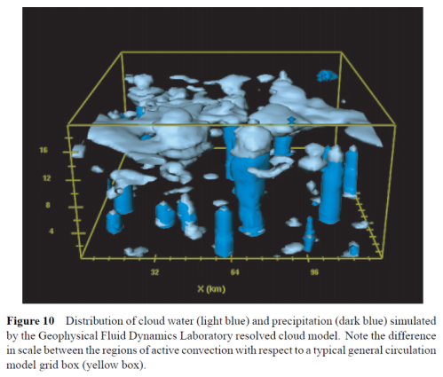
Held and Soden (2000)
Figure 1
The problem is, when you create a fudge factor you are attempting to combine multiple processes operating over different ranges and different times and get some kind of average. In the world of non-linear physics (the real world), these can change radically with very slight changes to conditions. Your model isn’t picking any of this up.
Here’s just one example from a climate science paper. It picks out one parameter in cloud microphysics, and uses three different values to run the climate model from 1860 to today and looks at the resulting temperature anomalies (see the last article 5 – Climate Models and Consensus Myths).
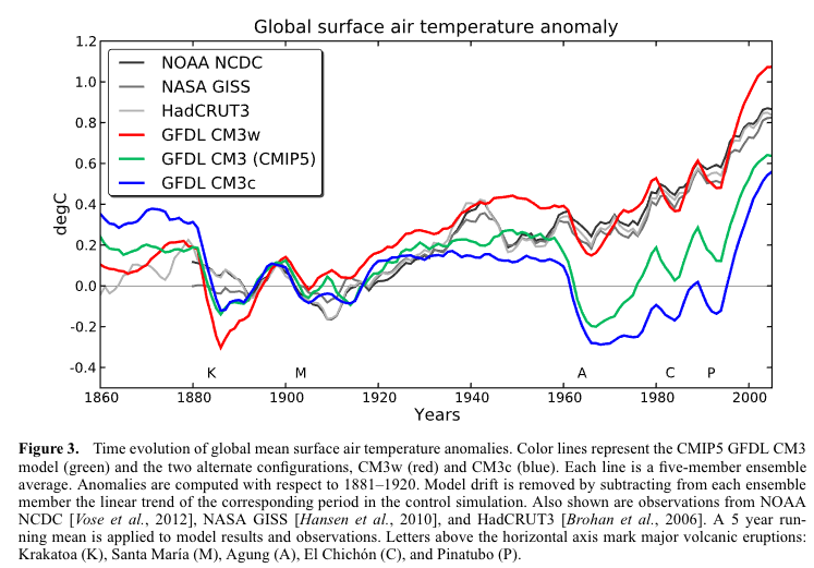
From Golaz et al 2013
Figure 2
The problem is that the (apparently) most accurate value of this parameter (blue) produces the “worst” result (the least accurate) for temperature anomalies. As the authors of the papers say:
Conversely, CM3c uses a more desirable value of 10.6μm but produces a very unrealistic 20th century temperature evolution. This might indicate the presence of compensating model errors. Recent advances in the use of satellite observations to evaluate warm rain processes [Suzuki et al., 2011; Wang et al., 2012] might help understand the nature of these compensating errors. (More about this paper in Models, On – and Off – the Catwalk – Part Five – More on Tuning & the Magic Behind the Scenes).
Conclusion
This is the reality in climate models. They do include giant fudge factors (sub-grid parameterizations). The “right value” is not clear. Often when some clarity appears and a better “right value” does appear, it throws off some other aspects of the climate model. And anyway, there may not be a “right value” at all.
This is well-known and well-understood in climate science, at least among those who work closely with models.
What is not well-known or understood is what to do about it, or what this means for the results produced by climate models. At least, there isn’t any kind of consensus.
Articles in this Series
Opinions and Perspectives – 1 – The Consensus
Opinions and Perspectives – 2 – There is More than One Proposition in Climate Science
Opinions and Perspectives – 3 – How much CO2 will there be? And Activists in Disguise
Opinions and Perspectives – 3.5 – Follow up to “How much CO2 will there be?”
Opinions and Perspectives – 4 – Climate Models and Contrarian Myths
Opinions and Perspectives – 5 – Climate Models and Consensus Myths
References
Cloud tuning in a coupled climate model: Impact on 20th century warming, Jean-Christophe Golaz, Larry W. Horowitz, and Hiram Levy II, GRL (2013) – free paper


Is ocean heat content a fudge factor?
https://tambonthongchai.com/2018/10/06/ohc/
No.
An example for the ocean is the vertical eddy diffusivity.
In doing a three-day weather forecast, are they using the same fudge?
JCH,
There are lots of differences between weather forecasting models and climate models. Also lots of similarities.
The underlying equation base is of course the same. Conservation of momentum, mass, heat and so on.
Three big differences that I see:
1. Much finer grid – I believe something like 1km x 1km for the best national weather forecasts vs 100km x 100km for climate models
2. Much shorter timescale to run over – a week or two vs a century
3. Opportunities for refinement based on results
The effect of 1 & 2 is the closure schemes – to solve “sub-grid parameterization” – are completely different due to the scales.
And I expect (but I don’t know the minute details of weather models) you don’t have to worry about drift in weather models. If the energy balance is incorrect then, for example, the temperature might drift by 0.002’C over 1 week. Unnoticeable. If the energy balance is incorrect by the same amount in a climate model the temperature will drift by 10’C over a century. So climate modelers and weather modelers are focused on very different outcomes.
The effect of 3 allows over-confidence, under-confidence to be reviewed and worked on.
So in weather forecasting you might run 50 models, with slightly different initial conditions and/or slightly different parameters (why?). Maybe 5 of the models say there is the chance of a severe storm. So you conclude that there is a 10% chance of a severe storm (5/50). The storm occurs. Were you correct in your 10% chance? You have no idea.
But over a year you look at all the 10%ers and see – did they occur roughly 10% of the time in reality? Or was it 30%? Or 2%?
So you can find out what you are over-confident of, or under-confident of, and attempt to find model changes which will make the model’s estimate of likelihood match up to reality.
I did write an article a while back which explains more on point 3 – Ensemble Forecasting.
SoD – thanks.
Niño 3.4 is below .5 ℃, so 18-19 El Niño is in a bit of trouble. For the moment anyway.
Another way to look at this is that pressure gradients in the atmosphere are usually low thus making Rossby waves relatively easy to model. However even in weather models there are issues such as the assumption that there is no turbulence outside the boundary layer. Thus the rate of decay of vortices and Rossby waves is determined by numerical viscosity. Much of the success of weather modeling is really doing a good job on Rossby waves over short time frames.
However even this success must be tempered strongly. If you ever read the forecast discussions the NWS does, you will see often something like “the models diverge at day 3” and we go with a broad brush forecast.
As SOD points out in the longer term, many other things become more important such as any lack of conservation of energy or tropical convection. Even weather models I suspect can’t predict tropical thunderstorms in detail very well. You might get a reasonable probability based on pressure gradients and past experience, but you simply cannot predict exactly where a thunderstorm will develop on any given day.
In the case of weather forecast models, we have the output from 700 model runs per year (with up to 50 different initialization) making predictions for every hour for two (?) weeks. With all of this data, we have a fairly good idea of how reliable a forecast is.
Climate modelers do not make “forecasts” intended to be validated by subsequent events. Look at the debates over Hansen’s early projections. Ever-evolving climate models are only checked by hindcasting, leaving open the possibility that models are tuned (intentionally or unintentionally) to agree with the past.
Thus we have the present stupid situation where negative aerosol forcing predicted by models is substantially stronger than now believed to be appropriate based on observations, and those wrong forcing estimates cause confusion in energy balance models. Two decades from now, we won’t be able to compare the projections of CMIP5 models with observed warming, because the realized forcings will not agree with forecast forcings included in various scenarios. CMIP output does not include the forcing produced by every driver. The other important potential “fudge factor” is ocean heat uptake, which allows any heat not escaping to space through an appropriately high climate feedback parameter to “disappear” into the deep ocean, and thereby not cause “too much warming” at the surface.
“All models are wrong. Some models are useful.” Today’s climate models are useful for encouraging policymakers to limit CO2 emissions. Candid discussion of validation might make them less useful for this purpose.
A few comments:
1) Arguments by arm-chair experts on blogs are not definitive. Bias/error analysis/predictability needs to be addressed quantitatively.
2) Errors go both ways. There is strong selection bias in making qualitative arguments. We all do it. However model bias can only be addressed by evaluating all the factors simultaneously, not by cherry-picking one or two to make a point. This takes well-designed studies. Emerging constraint studies are looking for bias and so far results haven’t indicated any high-side bias.
3) IMO the paleo record is the best way to estimate ECS. Our recent observational record certainly supports a sensitive climate.
4) Tuning is a feature not a bug. Based on the track-record established since the 1980s, reasonable forward projections can be made by tuning climate models. Tuning is not trivial. Think of it this way, tuning a climate model involves many orders of magnitude more information than a tuning a simple EBM.
5) The big picture needs to be considered. Models handle water vapor feedback well. If there was any way to avoid strong H2O feedback, models would be the way to demonstrate it. 2) There are certain cloud effects in a warming climate that are independent of sub-grid-scale phenomena, likely to cause warming and where models have skill. The list includes: convective clouds in the tropics extend to greater height; Hadley cells expand to the north, storm tracks shift to the north, low level cloudiness expands in the polar night as sea ice shrinks.
Well Chubbs, Sod is more than an “arm chair expert.” In any case, what he says here is in my view correct. Tuning is not a “feature”. It’s a messy way to try to overcome the fact that many scales of the flow are not resolved by the grid.
What you say about clouds is quantitative and as such does not help much in terms of determining cloud feedback or how to model clouds.
I’d like to see evidence that models handle H2O feedback “well.” There is some evidence that in the tropics they do OK on total column water vapor. But the distribution of that water vapor is important too. Stronger convection will affect that distribution.
Paleo estimates are all over the place. They are a lot less reliable than modern observational evidence.
Sorry, I meant to say that what you say about clouds is QUALITATIVE and NOT quantitative.
Chubbs,
Thanks for your kind words, but I think you are over-stating my knowledge. I am no expert.
It’s usually an office type chair as well, but that’s probably not important.
In this blog – at least up until this series – we try and see what scientific evidence exists for various claims. There are no authorities. Of course, I expect that people who write textbooks know what they are doing and that’s who I’ve learnt from. Likewise, climate scientists who have worked in a sub-field for decades and published 100 papers know 10,000x more than me on that sub-field so I read their papers and assume they understand the subject better than anyone else.
But in the end, all claims need to be evaluated – what evidence is there for a set of claims?
And in this article, you might have misunderstood. I’m not doing a treatise on climate models. I’m reviewing a website with what seems to be an overly positive message on climate models, aimed at the general public.
SOD
Sorry I certainly didn’t mean any offense. Also thanks for the clarification on the purpose of the blog article. I had completely missed it to be honest. Your article reads much more like a criticism of climate models than of another blog article.
Regarding evidence, I didn’t see any. Climate model output is understood to reflect to average conditions over a very large number of realizations. So yes, models will be wrong in every single grid square at every single time step. But you haven’t provided any information on model performance and the relative importance of sub-grid vs. other model physics. It may be that thermodynamics drive the key results. So don’t think this article says anything about the value or use of climate models or whether “fudge factor” is a good term to convey information about climate models to the public.
I close by linking a journal article from Manabe and Weatherald (1975) perhaps the first GCM, I am not sure. Many caveats from the authors, very primitive, no ocean, yet the findings in the abstract aren’t bad, old hat now. You have to hunt for the ECS which is buried, not far from CMIP5, I’m sure there were compensating errors.
https://journals.ametsoc.org/doi/10.1175/1520-0469%281975%29032%3C0003%3ATEODTC%3E2.0.CO%3B2
Chubbs, I really think you don’t understand the issue. If in fact hind casting of GMST is a result of tuning and other things like clouds or effective aerosol forcing or ocean heat uptake are wrong then overall energy flows are wrong and future projections will be wrong too.
So far you have dealt with a single integral output function and that means little in terms of skill.
You seem to be unaware also of the importance of the distributions of forcings and energy flows to ECS and TCR and ultimately temperatures. The ice ages were caused by changes in the distribution of forcing. The total forcing remained constant. That’s as close to a proof as you are going to get in this field.
With respect, SOD showed an example of the very large impact of cloud microphysics sub grid parameters on the global mean temperature in the GFL model. This proves that “thermodynamics” does not drive the result. Just as in all CFD, the dynamics are critical for overall forces and temperature.
Sorry I should have said that thermodynamics does not determine the outcome by itself. Dynamics are also critically important.
Sorry dpy I don’t think you know the issue. Model performance hasn’t been discussed here. You are arguing from incredularity. What seems incredible to you is SOP to me.
How do you know dynamics are important? Lets take ENSO for example; very important for this year, somewhat important for this decade, unimportant for this century.
Dynamics are critical in all CFD simulations including of the atmosphere. Dynamics for example determine the equator to pole temperature gradient, cloud feedbacks, and indeed the lapse rate. It’s an obvious point to people in the field.
Regarding dynamics – climate models do a good job of simulating average global circulation.
Here is a reference for my statement on models getting some of the large-scale cloud feedbacks right:
https://www.nature.com/articles/nature18273
Another opinion on water vapor feedback from Nic Lewis:
“There is more doubt about whether the combined water vapour + lapse rate feedback in AOGCMs is realistic, despite model estimates being fairly consistent at around +1.0 Wm−2 °C−1. This feedback is concentrated in the tropics, where AOGCMs simulate strong warming in the upper troposphere with specific humidity (the amount of water vapour), which has a particularly powerful effect there, increasing and absorbing more radiation. Saturation water vapour pressure increases rapidly with temperature, so this would happen if relative humidity were constant. Observational evidence does not appear to support the existence of such a strong tropical “hot spot”. This suggests that water vapour feedback (and the weaker, opposing, lapse rate feedback) may be overestimated in AOGCMs. The below chart27 compares tropical warming trends in CMIP5 models and various observationally-based datasets over recent decades. The 100000 Pa (1000 mb) pressure level is near surface level, 30000 Pa (300 mb) is in the mid-upper troposphere.
Related to this, although some evidence suggests specific humidity has gone up (with relative humidity changing little)28, as in most AOGCMs, other evidence suggests it has been steady or fallen,29 30. NOAA data31 shows a marked decline in tropical upper tropospheric water vapour over recent decades, although this represents a model-based reanalysis and may not be accurate.”
28 Chung E-S. et al, 2014. Upper-tropospheric moistening in response to anthropogenic warming. PNAS doi/10.1073/pnas.1409659111
29 Vonder Haar, T.H.,J.L. Bytheway, and J. M. Forsythe, 2012.Weather and climate analyses using improved global water vapor observations, Geophys. Res. Lett.,39: L15802, doi:10.1029/2012GL052094.
30 http://www.drroyspencer.com/2015/08/new-evidence-regarding-tropical-water-vapor-feedback-lindzens-iris- effect-and-the-missing-hotspot/ Also see graphs in http://www.friendsofscience.org/assets/documents/NVAP_March2013.pdf
31 NOAA ERSL water vapour data. Specific humidity, 300 mb, 30N-30S, 0-360E, monthly values, area weighted grid. 300 mb, the highest level available, is in the upper troposphere.
It is very difficult to evaluate water vapor feedback with observations. I have seen several flawed attempts in the past. The best analyses have come to the opposite conclusion. Below for instance:
https://www.pnas.org/content/111/32/11636.short
While difficult in observations, it is very easy to evaluate water vapor feedback in a model and model results are tightly clustered. Strong water vapor feedback has been a consistent result for decades. If there was a way to generate a lower water feedback by adjusting model physics, someone would have reported it by now.
To me Nick’s document sounds like advocacy, not science.
dpy,
The “friends of science” are an… interesting choice of citation.
From their website
“Our Opinion:
It is our opinion that the Sun is the main direct and indirect driver of climate change. ”
Unlikely to be a reliable source.
https://friendsofscience.org
Nit picking is not interesting VTG. The quoted document has many references. Can you respond to the substance of the point about effective feedbacks in models varying over a large range.
dpy,
the use of reputable sources is not “not-picking”, it’s central to good faith technical discourse. Please use reputable sources, not political websites with a self-avowed prejudged opinion.
I’m not sure what precisely you refer to in ” the point about effective feedbacks in models varying over a large range.”, as your comment doesn’t refer to this as far as i can see. Is this some new point? There is indeed a wide range in sensitivity due to uncertainty in feedbacks.
Well “reputable” sources are often wrong too. Nic has perhaps 40 references. Your selection of one you don’t like is not a valid point. Can you respond to the technical substance for once?
dpy,
I have no idea what you want a response on. I have already asked…
Chubbs, Nic’s point here is technical and it seems well sourced to me. The whole issue of water vapor is tied up in convection, precipitation, clouds, and the lapse rate. Models don’t do a good job at any of these except perhaps the last one. An obvious conclusion once again is that if indeed they agree with what meager and uncertain data there is out there, it is not due to skill but to fortuitous cancellation of errors in the sub grid models.
I checked one reference, 29. It presents a “new” globally merged TPW data set for the period 1989 to 2009. Much of the paper covers work to remove biases in the data sets that are merged. Note that the data period ends in a La Nina, that depresses TPW values. No trend analysis or even trend discussion is included. Here is a quote: “Therefore, at this time, we can neither prove nor disprove a robust trend in the global water vapor data.”
#30 comes from a court case so is an advocacy document, covers 1990 to 2001 and doesn’t show any impact of the 1998 el nino.
There are many other observational references that could have been cited here.
Nothing in Nicks document is quantitative regarding lapse rate and H2O feedback – purely qualitative.
On the flip side we have very little spread in model lapse rate/H20 feedback estimates and there are published studies which show observations are consistent with the models.
So unconvincing and frankly not worth the time to analyze.
Chubbs: Manabe and Weatherald (1975) contains grossly wrong prediction about many things. Compare Figure 10 to today’s KT energy balance diagram. This mistakes occurred because M&W couldn’t properly model the flux of sensible heat and latent heat from between land/ocean and the atmosphere using large grid cells. You were correct recognize the likely existence of compensating errors in parameterization and pay little attention to the model’s ECS.
However, today’s models still have the same problems: The grid cells are still vastly too large to properly model heat fluxes at the boundary between surface and the atmosphere (as well as between clear and cloudy skies). The biggest problem occurs with the boundary layer, which IIRC is only two grid cells high, and topped by boundary layer clouds (the most cooling clouds on the planet). Yet, for some reason, you now choose to ignore compensating errors and believe model ECS.
However, the same Manabe provides evidence that today’s models are still filled with compensating errors. The linked paper shows the large observed (CERES) and modeled feedbacks that accompany seasonal warming. Models do a poor job of reproducing the observed changes in LWR from cloud skies (observed feedback is insignificantly negative rather than positive) and the changes in SWR (which aren’t linear with temperature and therefore aren’t “feedbacks”). Even worse, models are mutually inconsistent. They have somewhat the same ECS due to compensating errors. Nevertheless, you choose to believe their predictions about ECS.
The feedbacks observed in seasonal warming may not be the same as those in global warming. Seasonal change is the net result of warming in one hemisphere and cooling in the other. It overweights feedbacks outside the tropics where the temperature change is the largest. Nevertheless, useful models should be able to deal with this situation.
https://www.pnas.org/content/110/19/7568
“Here, we show that the gain factors obtained from satellite observations of cloud radiative forcing are effective for identifying systematic biases of the feedback processes that control the sensitivity of simulated climate, providing useful information for validating and improving a climate model.”
Yes Frank, the compensating errors point is obvious from first principles as well as experience with the models. It is amazing to me that anyone with any modeling experience would not credit this point.
I think elsewhere I pointed to the Zhou et al paper on tuning cloud microphysics which showed that ECS could be engineered over a wide range using credible values of the sub grid model parameters. That’s about as clear an evidence of the compensating errors idea as any I’ve seen.
SOD, Great post.
One could look to turbulence modeling as an example of how to improve sub grid models.
In the 1970’s practical turbulence models were algebraic (like the climate sub grid models you describe here). The local value of eddy viscosity was determined from the local properties of the flow field. Later as computers advanced one was able to use more sophisticated models which are partial differential equations that are global that are solved simultaneously with the Navier-Stokes equations. These extra PDE’s produce the eddy viscosity. This resulted in a dramatic improvement in the quality of the modeling.
Of course there are still limitations that are well known for more challenging flows. The problem is that the model parameters are determined based on simple 2D correlations based on 2D wind tunnel testing. Thus, complex 3D flows are not going to be right even though they are often not as bad as one might expect.
Another problem is that the PDE’s being solved are strongly nonlinear so the equations become hard to solve and there are bifurcations, multiple solutions, etc.
But overall, the modern models are a vast improvement.
SoD you say:
“Depending on the group I might hasten to add that “giant fudge factors” isn’t a nasty term, aimed at some nefarious activity of climate scientists. It’s just to paint a conceptual picture to people.”
I have an educational background in engineering science, environmental engineering, and meteorology and I’ve heard the term “fudge factors” many times over the years and I have even made simple spreadsheet air quality forecast models using “fudge factors” that work fairly well. My understanding is that weather models are full of “fudge factors” and they work reasonably well out to a few days.
So I agree that “fudge factors” are not necessarily a bad thing. However, my experience in using fudge factors is that they ideally need to be determined based on actual measurements and then later adjusted based on model performance over time for best results. No complex model will ever be perfect, but most forecast models can be improved over time. I think the current crop of climate models have a LOT of room for improvement.
Oz4 – that is the question I asked above: do weather modelers have to do the same steps: making fudge? Climate models are often described as simply being weather models. I was thinking climate modelers probably have to do many of the same/similar steps.
I have a nephew who is working on his PhD in Quantum Computing. Even if he and his fellow researchers are successful, I doubt a quantum computer could run a climate model in the manner people seem to be expecting.
One problem here JCH is that weather models can use vastly finer grids for their simulations. But weather models take advantage of the fact that Rossby waves are an easy problem over short time frames. I doubt weather forecasts are very good in the tropics where there are usually scattered showers. But in climate, its critical to model the tropics well.
JCH, I’ve used the output from weather models for forecasting weather and air quality since I was in college at the University of Texas at Austin in the early and mid 70’s and I have watched them evolve over the years. Even in retirement now I still look at a variety of weather model forecasts daily. However, I’m no expert on how they work. I do know that global weather models like GFS and ECMWF do not have the resolution necessary to resolve convective thunderstorm cells. The current GFS resolution is 1 degree of latitude by 1 degree of longitude. So I’m guessing that finer scale features, like cloud convection must be parameterized. The GFS performs fairly well for large scale weather features, but has little to no skill at predicting smaller features like squall lines and meso-cell thunderstorms. The newer high resolution regional models, like HRRR and NAM 3km do attempt to resolve convective clouds and perform better than the global models in this regard, but suffer from relatively sparse high resolution vertically resolved input compared to the grid spacing. The UM CCI Climate Reanalyzer has a nice display of the NAM3 here (be sure to check out the different parameters):
https://climatereanalyzer.org/wx/fcst/#nam.conus-lc.t2
Oops … I goofed on the GFS resolution. It’s now half a degree latitude/longitude resolution, which is still not small enough to resolve clouds and convection.
For some people interested in weather and climate models, I recommend Representing model uncertainty in weather and climate prediction,
TN Palmer et al (2005) – free paper.
There are a couple of useful ways that sub-grid parameterizations (fudge factors) are developed:
1. Process studies
2. Higher resolution models
1. Observe some specific climate processes via lots of instruments in one area – you might have some boats out on the ocean, planes collecting data at certain altitudes, satellite data. Out of the dataset comes a parameterization scheme.
2. I give an example of this – Siefert et al 2015 – at the end of Models, On – and Off – the Catwalk – Part Five – More on Tuning & the Magic Behind the Scenes.
Lots can be learnt from these high resolution models.
Just a note that higher resolution models still need “closure schemes” (fudge factors) unless they can resolve down to the mm scale. If they could resolve down to the mm scale there would still be lots of uncertainties (we find that dust particle size affects this process, what is the dust particle size in area x,y,z.. and so on). The Siefert 2015 example had a 25m x 25m grid and ran for a simulated 60hrs.
The other way that fudge factors are developed is finding the best value to ensure the modeled climate does what the real climate does, or did.
One thing that puzzles me about these high resolution models is how they can possibly handle free air turbulence. This turbulence is highly variable and must have a significant effect on the global energy transfers. Normally one would use an eddy viscosity model but these are expensive and work rather poorly for things like free shear layers (at the edges of convective cells for example).
[deleted by capricious moderator]
I just looked up the Siefert post and they avoid eddy viscosity models by using LES. That answers my question.
The fact remains, weather models often work very well. I follow the 10 day global forecasts by an online reanalysis site. While not perfect, they’re pretty good. As month unfolds, you have a pretty good idea what the BEST and GISS, etc. anomalies will be.
Here is a recent paper which describes the slow but steady progress in weather forecasting over the decades. Behind a paywall unfortunately, but the reference list includes many of the important “fudge factors” which are also used in climate models.
https://www.nature.com/articles/nature14956
SOD already explained that weather forecasting and climate modeling are fundamentally different in their purposes and the grid spacings to name just one difference. Weather is about short term prediction of Rossby waves, a relatively easy problem. Climate is about energy flows and long term dynamics of the system with the tropics being very important. Weather model skill does not imply climate model skill.
The big difference between weather forecasting and climate modeling is that climate models only have to be right on the long-term average; not for next Tuesday’s weather forecast, so climate modeling is much easier than weather forecasting.
Sub-grid processes are critical to the accuracy of weather forecasts so climate models get to piggy-back on the technology developed for weather forecasting. The same “fudge factors” used in climate models are being run operationally at great expense around the world.
Chubbs, As i’ve mentioned several times, your view on this is not correct. Overall “averages” will change when the detailed dynamics change. For example if convection becomes stronger that will create a change in the vertical temperature structure and humidity structure that will change the outgoing radiation balance.
Here’s another paper finding the importance of dynamics in climate.
https://ams.confex.com/ams/2019Annual/meetingapp.cgi/Paper/354779
Your reference indicates that using measured SST instead of model predicted SST improves the prediction of precipitation and vertical velocity. That seems very reasonable to me. Actual gradients are more intense than modeled. That also seems reasonable. Doesn’t say anything about ECS, though.
Here is a somewhat relevant example from weather forecasting. Weather models use ensemble forecasting methods where the initial conditions and/or the model physics of a best case operational model are perturbed to generate a range of possible outcomes. It is almost always the case that the average of the ensemble is a better forecast than the unperturbed operational model; even though, the operational model has better data and physics than any of the individual ensemble members.
[…] « Opinions and Perspectives – 6 – Climate Models, Consensus Myths and Fudge Factors […]
SoD,
“In the least technical terms I can think of.. imagine that we divided the world up into a 3d grid. Our climate model has one (and only one) value in each cell for east-west winds, north-south winds, up-down winds, high cloud fraction, low cloud fraction, water vapor concentration.. basically everything you might think is important for determining climate.”
You’re omitting something important here. GCM’s, as in CFD, are solving the Navier-Stokes equations. That is, the equations for momentum and mass, and also an accounting for energy. The essential point is that these are conserved quantities. That is, there is a meaningful mass and momentum for a cell. Just one number. And the N-S solution process balances that, basically by accounting at boundaries (boundary forces and fluxes).
That is the PDE solution process. The other things are subsidiary things that you can carry along. To take one interesting example that you mention – vertical velocity.
In fact, GCM’s radically simplify (for good reason) the vertical component of the momentum equation. They use a hydrostatic balance. This isn’t overwriting N-S with something new. It is just using the terms that remain when you say that the forces associated with vertical acceleration, and that component of viscous shear, are negligible. So they can be dropped from the force balance, leaving g and pressure gradient. That isn’t to say that vertical transport is impossible. We know it happens in storms, especially hurricanes etc. But we know too that these are infrequent. So they have an updraft model to account for that transport. That isn’t affecting the basic N-S solution process, which is the rapid time change process. It says that you can observe what happens, and add it in as a corrector.
I think Nick that the numbers for a given cell will be badly wrong if the cells are too big because of large numerical truncation errors.
Most CFD methods do discretely conserve mass, momentum, and energy. That’s not however always the case for climate models as i understand it. This conservation helps accuracy but is no guarantee of accuracy.
Generally, one needs sub grid models for scales not resolved by the grid. That’s where the fudge factors come in.
There is a strange side of models that Clive Best has put some light on, in his blogpost. “A comparison of CMIP5 Climate Models with HadCRUT4.6” Where he shows a comparison of the latest HadCRUT4.6 temperatures with CMIP5 models for Representative Concentration Pathways (RCPs). The temperature data lies significantly below all RCPs, which themselves only diverge after ~2025.
He has calculated Global Surface temperatures from 12 different CMIP5 models run with RCP8.5 from 1860 to 2100. These runs give a remarkabe result: There is a huge disagreement on the global average surface temperature even in 2018– a spread of 4C. The models now spread from a little over 12 deg C to a little over 16 deg C. This means a great cooling bias in most of the models. So, when the models get used, they must be adjusted to the real temperatures which are measured today? Some kind of fudge gymnastics.
NK: Basically, you are asking if models that get pre-industrial temperature wrong can predict the right amount of warming from 2XCO2?
For pre-industrial in a simple zero-dimensional model:
S(1-a) = eoTs^4 = 240 W/m2
If models get Ts wrong, then they must get the planet’s effective emissivity (e) or albedo (a) wrong T=288, e = 0.614 and Ts=289, e = 0.0607 both give 240 W/m2, so the “error” is actually very small. We have a pretty good idea of how much energy is being delivered by the sun (S) and it appears fairly constant, so let’s assume it isn’t one of the things that might be wrong.
RCP’s specify a given radiation forcing (say 8.5 W/m2), so there is no error in forcing. To calculate warming at steady steady, you need to know planet’s climate feedback parameter (dRi/dTs), the change in radiative imbalance (Ri) per degK of surface warming.
Ri = S(1-a) – eoTs^4
dRi/dT = -4eoT^3 – (oTs^4)*(de/dTs) – S*(da/dTs)
In other words, can models that get a or e very slightly wrong be trusted to get da/dTs and de/dTs right? As best I can tell, the former has no bearing on the latter.
Thank you for the clarification, Frank.
Could fudge factors be about neutralizing sysrematic errors in models?
According to Wild et al , 2014: “The magnitudes of TOA fluxes over land and oceans can now well be determined from the CERES satellite observations. The CMIP5 multimodel mean solar and thermal fluxes closely match these observations when averaged over land and oceans. More substantial biases remain in individual models. Compared to the TOA fluxes, the magnitudes of the surface fluxes are much less well established, as they are not directly measurable by satellites. Historically, this has lead to an unsatisfactory large spread in the surface flux estimates already on global or land/ocean averaged-scales, and has prevented the establishment of firm agreed-upon reference values for the magnitudes of the ocean and land surface energy balance components. This is still evident in the significant spread in the land and ocean surface budgets of the CMIP5 models. Compared to direct surface observations, the majority of these models tend to overestimate the downward solar radiation over land and oceans, and underestimate the downward thermal radiation particularly over land.”
The energy balance over land and oceans: an assessment based
on direct observations and CMIP5 climate models
Martin Wild · Doris Folini · Maria Z. Hakuba · Christoph Schär ·
Sonia I. Seneviratne · Seiji Kato · David Rutan · Christof Ammann ·
Eric F. Wood · Gert König‑Langlo
Click to access 10.1007%2Fs00382-014-2430-z.pdf
So ,even solar radiation at land and ocean surface is wrong in models, and show very different values across models. The same with downward thermal radiation. But why bother when they go in opposite direction. And in addition we can bring in some fudge factor to balance it even more. So, let us calculate the climate in year 2100 with neutralized systematic biases. And if Martin Wild protests, he can be neutralized at RealClimate.
Wild, PowerPoint Presentation
Click to access 13369-verification-radiation-large-scale-climate-models.pdf
I think this is overly negative about climate models. While there are tunable parameters in the models, that does not mean that you can get anything you want out of a model. One thing that has had a big influence on me is the research that sweeps parameter space of the models to determine the range of climate sensitivities that one can reasonably get from a model. They find that ECS > 2 in just about any realistic model (e.g., models must be stable).
Click to access nature_first_results.pdf
It’s also worth saying that people spend an incredible amount of time refining parameterizations. As a result, the models do an incredible job at many things that rely on these, like the water vapor feedback.
I think Andrew you may be suffering from selection bias. There are lots of things the models get wrong. Regional precipitation is one SOD showed here. TLT is another one. It seems that the vertical temperature profile in the tropics is also badly missed. Convection aggregation is shown by experiments to reduce ECS quite significantly and is mostly not accounted for. There was a paper looking at solar flux at the surface. It was off in models by an average of 7 W/m2. Cloud fraction as a function of latitude is all over the place. Gavin Schmidt just posted on the ocean heat uptake in the GISS model which appears to be significantly higher than the most recent data analyses show. These things lend credence to the fudge factor characterization.
I can relate this to the history of turbulence modeling where big steps forward have been taken. Most climate sub grid models are algebraic like practical turbulence models were 40 years ago. The results were generally poor. Modern models solve global PDE’s for the eddy viscosity and are a lot better. It is very unlikely that convection in one grid cell doesn’t impact neighboring grid cells.
First principles analysis shows that the numerical truncation errors in climate models are very large. Also sub grid models for convection are also almost certainly way off. The only way you can get skill on some measures in these circumstances is if what you are looking at is strongly related to quantities used in tuning. That tuning merely optimizes cancellation of errors.
If you read here in the comments and elsewhere you will find some of the references to negative results. One that shocked me was the extreme sensitivity of model results to the order in which sub grid models are applied. What that means is that these models are not independent of numerical details and so tuning will become wrong when those details change. If I had such a low standard for CFD modeling, I’d be fired.
https://agupubs.onlinelibrary.wiley.com/doi/full/10.1002/2017MS001067
Here’s another one.
https://journals.ametsoc.org/doi/10.1175/JCLI-D-15-0191.1
In figure 1 of your reference Andrew, there are some (only a few though) model runs for a doubling CO2 scenario that have decreasing temperatures.
It seems to me that regional and continental scale predictions are the real supposed value of climate models. Energy balance methods can also project average temperatures quite well. While it is true that effective forcings are needed, those are globally averaged forcings. As we get better data on ocean heat uptake, TOA radiation imbalance and forcings, those simple model predictions will get better.
In fact even on the measure of global average temperature anomaly the model performance is not great. Here are some plots by Clive Best.
Here’s one comparing models vs. reanalysis data from weather modeling.
This was in response to Zeke Hausfather tweeting a graphic showing almost perfect agreement of CMIP5 with data but using a baselining period of 1981-2010. Clive used 1961-1990 which is what AR5 used and what the Hadley center uses. This just shows that there is a lot of stuff that gets out there that doesn’t hold up under careful analysis.
So, the bottom line question is why all the continued huge investment in climate models when they add little to our ability to predict anything? Given the very coarse grids used and the algebraic sub grid models (which experience in turbulence modeling shows are unlikely to be very good), is there any prospect that they will become skillful anytime in the foreseeable future?
Seems to me that better data and better theory will give more information for the dollars invested. Aeronautical CFD is hard enough already. There is at least some prospect that continued investment will improve CFD skill because the models are already pretty good for many situations and the deficiencies better understood. This will give us a better handle on how to improve climate models.
“First principles analysis shows that the numerical truncation errors in climate models are very large. Also sub grid models for convection are also almost certainly way off. The only way you can get skill on some measures in these circumstances is if what you are looking at is strongly related to quantities used in tuning. That tuning merely optimizes cancellation of errors.”
Even if you use something like LES to simulate the large scales and make use of the fact that backscatter is very small and energy flows in the mean to the smallest resolved scales, you will have almost no chance in getting the subgrid information you would like to have with big grid cells.
People tried to use stochastic models to generate some structure mimicking some kind of isotropic turbulence. Nevertheless, trying to find accurate prediction on the subgrid scale is impossible, in my opinion, esp. for higher moments. I say so doing those simulations for years and developing models myself.
Most one- or two-equation RANS models are a lot worse, relying on crude eddy viscosity concepts with often only one external length scale. Those models, when applied to wings etc., are perfectly able to get integral quantities reliably (e.g. drag or lift, used by the big car and air-plane companies), but fail already in prediction detachment or reattachment, reliably. As you said, Reynolds stress models have become really good but due to the higher cost aren’t used in industry at all – I know of no German manufacturer having used any for production stuff. Nevertheless I consider those important, as they are able to deal with anisiotropy.
The problem is not, that those RANS models lack physics. It is that the physics involved is often crude or simplified, lacking important mechanisms and therefore not being able to predict strongly anisotropic turbulent flows requiring a multitude of length and time scales.
LES is a much better way to go and my experience is that you get excellent results, but only if you can afford the computational expense and resolution required to resolve the high shear/gradient regions and have a mesh of the order of the scales you want to make predictions about.
Yes Holger sounds like you have a lot of experience. However, there are problems with LES too. My sources tell me that there is no grid convergence and that there is sensitivity to initial conditions too. What I’ve seen so far is pretty sketchy and isn’t really very convincing.
Andrew,
Welcome.
What do you think about the paper by Golaz?
I know Chris and I trust his work. As the paper points out, there remain important problems in understanding the temperature evolution of the 20th century, and the magnitude of aerosol indirect forcing is one of the biggest. Nevertheless, that doesn’t really negate my point that no one has demonstrated that you can tune the parameters in a model to get a very low ECS (i.e., much less than 2 deg). It may be possible, of course, but it’s yet to be demonstrated. Combined with other results from measurements of feedbacks based on observations & simple theoretical arguments, the case for ECS < 2 deg is, in the opinion of most experts, weak.
Andrew,
I’m not making that point in this article. That is, I’m not claiming anything about the likely ECS range (and as best as I understand the work of climate science so far I believe you are correct).
This article, this series, is aimed at a less technical audience. A previous article commented on contrarian myths on climate models. The last article and this one comment on “consensus myths” (where “consensus” = popularized support for the climate science position).
The myths:
– there aren’t fudge factors in climate models
– reproducing past global temperature anomalies means that “we can trust climate models”
Regardless of how few people read this blog, I’m trying to explain important subtleties of climate science. This series is more a commentary.
—
But interesting questions follow in my next comment..
interesting questions..
– in reading a large number of papers on the ice ages I found that as model refinement improved, a proposition that seemed supported became unsupported, then supported again with yet more model improvement (onset of ice ages with year round snow cover at high latitude)
– likewise in reading papers on improved model resolution in the oceans (over a much smaller domain) I found that clarity appeared where in coarser models the simulations had more problems.
So, I wonder.
At the moment we can simulate century scale at 100km x 100km. When we can simulate the same time scale at 1km x 1km (if we ever can) how will this change projections of precipitation, regional temperature changes, and so on?
How can we have confidence in models that disagree on regional changes yet it appears regional changes matter for model predictions? (I can expand on this question, but will need to look up a bunch of papers, hopefully you see where I am aiming).
I think the answer is that I wouldn’t put a lot of faith in specific regional predictions of climate models for 2 reasons. First, it’s not clear that the models are capable of doing that, and second, internal variability can have huge impacts on regional climate (http://www.cgd.ucar.edu/staff/cdeser/docs/deser.communicating_navari.ncc12.pdf), so that even with a perfect model, to get internal variability right you also have to initialize the model perfectly, too.
Overall, I think people should be skeptical of models. We are not confident of our future predictions because we are confident in the models. Rather, the field relies on observations and simple physical arguments. Models are useful to verify those and to allow us to better understand phenomena. Water vapor feedback is a good example: our extremely high confidence is based on simple physical arguments (https://journals.ametsoc.org/doi/pdf/10.1175/JCLI-D-14-00255.1) and observations (https://drive.google.com/file/d/0ByXC85Z909PTNm42ZzE4Zk5SVzQ/view). The fact that models simulate it correctly adds to our confidence.
So what can we say about regional temperature changes? We know temperatures are going up everywhere — more on land than ocean and more in winter and at night than summer and the day. And more in the middle of continents than on the edge. Those conclusions arise from simple physics. We know that, as the Earth warms, the jet streams will move poleward as the Hadley cell expands, which is another simple physical argument. This will push precipitation poleward. You don’t need climate models to reach any of these conclusions.
If you want to know what’s going to happen to your hometown, I don’t think we’re in a position to say that yet.
How about continent?
For continents, I think the models are going to do a reasonable job. That said, internal variability is important for predictions at that scale, so you not only need a good model, you also have to initialize the model with an accurate state of the ocean. I suspect that the initialization is a much bigger roadblock to regional predictions than the parameterizations of the model.
I really recommend this paper: http://www.cgd.ucar.edu/staff/cdeser/docs/deser.communicating_navari.ncc12.pdf
It’s quite good and really shows how internal variability confounds regional predictions.
And yet for Australia the average rainfall over 25 years, as hindcast by the various modeling groups, shows a large range compared with reality. At least double through to less than 50% (see last article).
I haven’t dug into the projections but my understanding is that even for RCP8.5 (my name “an extreme emissions scenario”), where we would hope to separate the signal from the noise, the 2100 projections have some models with large increases in rainfall and some with large decreases in rainfall, and everything in between.
It doesn’t seem like a reasonable job for Australia. I know it’s a small place.
I haven’t looked into Australian rainfall so I don’t know if there are any rigorous results there. From a policy perspective, it may be that all you can say is that you need to be prepared for large, but unspecified changes in precip under high emissions scenarios. It’s worth noting that regional rainfall is hard, but that doesn’t mean that we know nothing about the future. If you want to know what you can “take to the bank,” you can bet on warmer temperatures in Australia, higher sea level, and acidified oceans.
Andrew said:
Thanks, it’s very interesting.
The paper you referenced Andrew is indeed very interesting and looks like a pretty strong negative result. Unless I’m misunderstanding, it looks to me as if models are all over the place even with regard to rates of temperature change over the next 40 years for the US, with some runs showing no change in the US and some a rapid rate of change. Summer seems a little bit more tightly clustered. Looks like Mazatlan has a much tighter range though with not much change being shown. This does not look like it can be blamed on internal variability to me since the trends look rather consistent over 40 years.
The global average temperature seems to be more tightly clustered. What that tells an experienced modeler is that the average is right perhaps because of conservation of energy (TOA radiation in is a tuned for metric and ocean heat uptake is in the ballpark) but the pattern is wrong in detail. That’s what is called in the trade cancellation of large errors. Experienced CFD modelers also know that in such a circumstance, output quantities will only be accurate either by chance or because they are related to quantities for which the model has been tuned.
With due respect, no one would use such poorly performing CFD models for decisions where human life or safety was involved. The FAA wouldn’t allow it and competant executives would never take such risks. Individual scientists would not allow it either or indeed present the results as if they were accurate or even meaningful.
Until recently, the GFDL models didn’t have the ability to produce and aerosol indirect effect. The Golaz paper explored parameterizations that introduce different amount of aerosol indirect effect into their models. Figure 2 shows that nothing else was improved or changed between three versions of CM3, but aerosol forcing changed: -1.0, -1.6 and -2.3 W/m2. (vs Total GHG forcing +2.6 W/m2.) Only about -0.5 W/m2 is reflection of SWR by aerosols. So now the CM3 model has parameters that can be tuned to hindcast whatever historic forcing one needs to make warming agree with observations without changing anything else about how the model functions. As SOD says, a giant fudge factor. (Since RCPs assume aerosol forcing is going to disappear, tuning the aerosol indirect effect has no future projections.)
Ironically, as Golaz (2013) was being published, the AR5 was casting extreme doubt about the ability of climate models to produce a realistic aerosol indirect effect.
7.4.3.1 The Physical Basis for Adjustments in Liquid Clouds (p609)
“The traditional view (Albrecht, 1989; Liou and Ou, 1989) has been that adjustment effects associated with aerosol–cloud–precipitation interactions will add to the initial albedo increase by increasing cloud amount. The chain of reasoning involves three steps: that droplet concentrations depend on the number of available CCN; that precipitation development is regulated by the droplet concentration; and that the development of precipitation reduces cloud amount (Stevens and Feingold, 2009). Of the three steps, the first has ample support in both observations and theory (Section 7.4.2.2). More problematic are the last two links in the chain of reasoning. Although increased droplet concentrations inhibit the initial development of precipitation (see Section 7.4.3.2.1), it is not clear that such an effect is sustained in an evolving cloud field. In the trade-cumulus regime, some modelling studies suggest the opposite, with increased aerosol concentrations actually promoting the development of deeper clouds and invigorating precipitation (Stevens and Seifert, 2008; see discussion of similar responses in deep convective clouds in Section 7.6.4). Others have shown alternating cycles of larger and smaller cloud water in both aerosol-perturbed stratocumulus (Sandu et al., 2008) and trade cumulus (Lee et al., 2012), pointing to the important role of environmental adjustment. There exists limited unambiguous observational evidence (exceptions to be given below) to support the original hypothesised cloud-amount effects, which are often assumed to hold universally and have dominated GCM parameterization of aerosol–cloud interactions. GCMs lack the more nuanced responses suggested by recent work, which influences their ERFaci estimates.
Figure 7.19 (p619) summarizes all of the available information about aerosol forcing and I will try to paste it below. If you believe models should reflect what we can measure from space, aerosol forcing should be from -0.45 to -0.95 W/m2 and only CM3w (-1.0 W/m2) is plausible. If you follow the IPCC’s expert judgement, CM3 (-1.6 W/m2) is on the edge of plausibility.
Figure 7.19 | (a) GCM studies and studies involving satellite estimates of RFari (red), ERFaci (green) and ERFari+aci (blue in grey-shaded box). Each symbol represents the best estimate per model and paper (see Table 7.3 for references). The values for RFari are obtained from the CMIP5 models. ERFaci and ERFari+aci studies from GCMs on liquid phase stratiform clouds are divided into those published prior to and included in AR4 (labelled AR4, triangles up), studies published after AR4 (labelled AR5, triangles down) and from the CMIP5/ACCMIP models (filled circles). GCM estimates that include adjustments beyond aerosol–cloud interactions in liquid phase stratiform clouds are divided into those including aerosol–cloud interactions in mixed-phase clouds (stars) and those including aerosol–cloud interactions in convective clouds (diamonds). Studies that take satellite data into account are labelled as ‘satellites’. Studies highlighted in black are considered for our expert judgement of ERFari+aci. (b) Whisker boxes from GCM studies and studies involving satellite data of RFari, ERFaci and ERFari+aci. They are grouped into RFari from CMIP5/ACCMIP GCMs (labelled CMIP5 in red), ERFaci from GCMs (labelled AR4, AR5 in green), all estimates of ERFari+aci shown in the upper panel (labelled ‘All’ in blue), ERFari+aci from GCMs highlighted in the upper panel (labelled ‘Highlighted GCMs’ in blue), ERFari+aci from satellites highlighted in the upper panel (labelled ‘Highlighted Satellites’ in blue), and our expert judgement based on estimates of ERFari+aci from these GCM and satellite studies (labelled ‘Expert Judgement’ in blue). Displayed are the averages (cross sign), median values (middle line), 17th and 83th percentiles (likely range shown as box boundaries) and 5th and 95th percentiles (whiskers). References for the individual estimates are provided in Table 7.3. Table 7.4 includes the values of the GCM and satellite studies considered for the expert judgement of ERFari+aci that are highlighted in black.
Andrew, on that subject:
It just occurred to me that if you ran the model shown in Golaz’ paper with the “realistic” value of the parameter (which shows no 20th century warming), maybe you would get no 21st century warming for RCP6?
I’m not sure what that tells anyone..
dpy6629,
I think you are misunderstanding it.
It’s one model with many runs, all starting from slightly different initial conditions.
The issue identified by the Golaz paper is with the aerosol indirect effect. Almost all of the forcing in the RCP’s is from greenhouse gases, so I’m confident that the warming over the 21st century would not be impacted much by the choice of how the indirect aerosol effect is parameterized.
Thanks SOD. That is surprising to me though. I would think that a 40 year consistent increasing trend of temperatures over the US of about 2C would be very rare. I do question whether real internal variability can be that large for example in the winter months. The historical US temps seem to follow pretty well the global values with admittedly more short term noise. But on 40 year periods, trends look pretty similar to me. Is an increase from 0 to about 4 in 40 years really possible when global temperatures only go about 1 degree?
From NASA Earth Observatory, 2004: “The scientists found that most climate models have been overestimating the amount of water vapor entering the atmosphere as the Earth’s surface warms.”
Another systematic bias.
Ha ha. You should look up who “The scientists” are and read the paper; that was not a very good description of the actual content of the paper.
Climate models are simulations. They are tuned to get global surface temperatures and TOA radiation right. I have never seen that they have a good grip on hydrological circle, as Hadey cell extension, upper tropospheric drying, precipitation and many other matters. These are the components of water vapor feedback.
And climate model runs are hypothesis, not evidence.
From a paper:Zachary Pirtle, Ryan Meyer, , and Andrew Hamilton, 2010: What does it mean when climate models agree? A case for assessing independence among general circulation models .2010.
“Climate modelers often use agreement among multiple general circulation models (GCMs) as a source of confidence in the accuracy of model projections. However, the significance of model agreement depends on how independent the models are from one another. The climate science literature does not address this. GCMs are independent of, and interdependent on one another, in different ways and degrees. Addressing the issue of model independence is crucial in explaining why agreement between models should boost confidence that their results have basis in reality.”
This is an excellent point. Most of the world’s climate really derive from less than half a dozen sources and the methods in the dynamical cores are pretty similar too. GFDL may be an exception in that they went to a Colella and Woodward discretization scheme instead of high order finite differences.
I just got a voicemail from someone (I won’t name them) thanking me for commenting on the blog. I’m glad that people appreciate my POV — sometimes it hard to know if anyone is listening. They didn’t leave any contact info, so I thought I’d say “thanks” here.
Hi Andrew, I appreciate your participation here as well. I haven’t met you before, but I have worked with your cohort John N-G in conjunction with several air quality studies in the past. Even though I would probably be best characterized as a climate “luke warmer”, I like to hear scientific arguments from all sides of the issues. No one person can know everything in this very complicated field.
I’ve been following weather models since I was studying meteorology in the now defunct UT Atmospheric Science Department with Professors Ken Jehn and Norm Wagner back in the early and mid 1970’s. The weather models have certainly come a long ways since back then. In retirement now, I’m trying to learn a bit more about weather and climate models, so your expertise is appreciated in that regard.
Delighted to see you back here, hope you stay engaged.
Well the paper on regional climate model ensemble predictions was interesting. Are there any comparisons with regional historical trends vs. historical model simulations for the region? There must be somewhere. I really question if on decadal time scales there is that much real internal variability. Particularly for winter in Seattle for example, it’s rare in my experience to have more than a few warm or cold ones in a decade. And decadal averages I am guessing would be pretty close to the underlying trend line. But maybe I’m wrong on that.
Likewise – good to see you back here and I hope you can hang around for a while. And thanks for the pointers to the paper above.. Interesting reading that!
I likewise appreciate your engagement. Given the natural tendency of humans to divide into tribes and be unable of assimilate evidence that contradicts deeply held beliefs, the only way even the most open-minded can really learn is by hearing the best arguments from all sides.
So far, I haven’t heard any compelling objections the thesis of this post:
“This is the reality in climate models. They do include giant fudge factors (sub-grid parameterizations). The “right value” is not clear. Often when some clarity appears and a better “right value” does appear, it throws off some other aspects of the climate model. And anyway, there may not be a “right value” at all.”
In the case of Golaz (2013), we see that hindcast warming can be dramatically changed by tuning the aerosol indirect effect, but mostly by creating an aerosol indirect effect which AR5 believes is too large and not supported by observations.
I agree with much of the Golaz paper: the aerosol indirect effect is one of the big uncertainties in climate science, and it’s one reason that we don’t really know what the historical radiative forcing is. That, in turn, is a primary reason the uncertainty in ECS estimated from the 20th century is so large.
However, we can also estimate ECS from periods where changes in forcing is not important (i.e., the last few decades), so we can end-run around this problem. https://drive.google.com/open?id=1OVUO_e6H5WMxhAYJhLiimY5kGYeL_Nyu
Second, aerosol indirect forcing is important to the 20th century forcing budget, but it is unimportant for the 21st century because it is completely dominated by CO2. So uncertainty in this will not cause much uncertainty in future warming.
At the risk of spoiling the good feelings here I should point out that this latest paper of Andy’s builds on an earlier paper with Mauritsen and Stevens (also from 2018) that Nic Lewis has critiqued in great detail. It appears to me that some of the criticisms are valid and may affect the later sections of the referenced paper too.
In Andy Dessler’s latest paper, Figure 1b shows a scatter plot and linear regression with Ts as the independent variability and R-F as the dependent variable, where F is radiative forcing and R is the imbalance at the TOA. (R = F + lambda*Ts, and the regression affords lambda, the climate feedback parameter and then ECS.) All variables are expressed in terms of monthly anomalies. R^2 shows that only 3% of the variance in R-F is explained by the change in Ts! As spoiled scientists who has had the satisfaction of performing well-controlled experiments in the laboratory, I personally find it absurd to assign any meaning to a regression based on an R^2 of 0.03 – despite the fact that similar plots have been published by many climate scientists of all persuasions.
If one looks at the TOA response to seasonal warming (Tsushima and Manabe (2013) PNAS), it is easier to understand why the regression in Figure 1 is likely meaningless. GMST (not the anomaly) seasonally rises 3.5 K every year due to the lower heat capacity of the NH and that produces unambiguous large changes in radiation at the TOA
The globally averaged, monthly mean TOA flux of outgoing longwave radiation (W/m2) over all sky (A) and clear sky (B) and the difference between them (i.e., longwave CRF) (C) are plotted against the global mean surface temperature (K) on the abscissa. The vertical and horizontal error bar on the plots indicates SD. The solid line through scatter plots is the regression line. The slope of dashed line [is 3.21 W/m2/K, Planck feedback with no other feedbacks]. https://www.pnas.org/content/pnas/110/19/7568.full.pdf
For LWR, we observe an unambiguous LINEAR signal showing that the planet as a whole emits about 2.2 W/m2/K more LWR from both clear and all skies (formally -2.2 W/m2/K) as it warms. In other words, WV+LR feedback is about +1 W/m2/K, and there is no positive cloud LWR feedback visible in this system (contrary to what AOGCMs predict). This is the kind of analysis anyone can trust.
Now let’s look at the SWR signal:
The globally averaged, monthly mean TOA flux (W/m2) of annually normalized, reflected solar radiation over all sky (A) and clear sky (B) and the difference between them (C) (i.e., solar CRF) are plotted against the global mean surface temperature (K) on the abscissa. The vertical and horizontal error bar on the plots indicates SD. The solid line through scatter plots is the regression line.
Now we clearly don’t have the same kind of SIMPLE linear relationship between reflected SWR (OSR) and Ts. Figure 2B shows the SWR response seen through clear skies, which is presumably the result of a combination of Rayleigh scattering (presumably independent of Ts) and surface albedo. Surface albedo change presumably reflects changes in seasonal snow cover sea ice. We EXPECT such responses to lag behind monthly Ts, explaining why we don’t see the same sort of unambiguously linear relationship we do for LWR. (The global sea ice anomaly shows two peaks per year during June and September and a single minimum in March, while snow cover is greatest during late winter in the NH.) Other factors may also be involved. It is clear that the response of cloudy skies at least partially lags behind monthly Ts, but the reason for this phenomena is less obvious. Lindzen and Choi and separately Spenser asserted that there is a slightly stronger correction between negative cloud feedback with a 3-month lag than the positive feedback observed with no lag. From my personal perspective, I think it is ludicrous to assert that any simple direct or lagged relationship describes the relationship between reflected SWR and Ts at ANY particular time. Emission of LWR is a function of Ts for obvious physical reasons, but there is no obvious reason to expect a simple physical relationship between reflection of SWR and Ts on a monthly time scale.
Dessler and Forster (2018) only analyze the sum of the LWR and SWR responses (R) to Ts and ignore the obvious fact that the SWR response can not be a simple function of the current monthly Ts anomaly. I don’t think this can tell us anything useful about the SWR feedbacks in response to global warming. The dynamic range of the temperature and radiation changes is much smaller and not reproduced every year.
Seasonal warming is the result of warming in the NH, cooling in the SH and relatively little change in the tropics, and therefore it is a lousy model for global warming. Nevertheless, it is obvious that AOGCMs are incapable of reproducing the large responses (except WV+LR through clear skies) to seasonal warming observed from space. Furthermore, those responses are mutually inconsistent between models.
Mauritsen and Stevens (2015) have recently confirmed the finds of Lindzen and Choi showing the that the LWR response to warming in the tropics shows POSITIVE LWR feedback (-4 W/m2/K). Our climate system is obviously much too complicated to be understood in terms of a single instantaneous (on a monthly time scale) global OLR+OSR response to changing Ts.
Click to access 553630ea0cf218056e92e697.pdf
Dessler and Forster do show a somewhat tighter correlation between the temperature at 500 hPa and R-F. Unfortunately, this is the temperature at 500 hPa from 30S-30N compared with global R-F. There is no physical rational for this pairing the data in this manner. When the authors eventually decide to compare tropics to tropics and non-tropics to non-tropics, separate the LWR and SWR channels and clear and cloudy skies, then it might be worth looking into the validity of their method for converting warming at 500 hPa into warming at the surface.
Suffice it to say I don’t agree with Nic Lewis. What we showed in Dessler, Mauritsen, and Stevens is that a model with an ECS of ~3°C could nevertheless look like an ECS of 2°C-4°C. Nothing he does in his analysis contradicts that.
He pushes forward a red-herring by focusing on changes in the uncertainty range (“this doesn’t change the uncertainty range”), and he’s right that if you add this in quadrature with other errors it has a small effect. But he doesn’t talk about how it effects the “most likely” value — it can move it by a significant amount.
When you add uncertainty to that issues with masking and blending of the observational surface temperature record (https://drive.google.com/file/d/1_C41ryDcWwq6bfNa22Lx8Z_b1MexROsY/view?usp=sharing), which also tend to low bias observational estimates by about 20%, the case that models are running hot begins to vaporize.
As far as the low R^2 criticism — yes, that’s a bummer. I wish we had more data so we could better isolate the signal. However, it is important to remember that low R^2 is not equal to high uncertainty … in fact they are unrelated. In the paper, we do a thorough uncertainty analysis and propagate the uncertainty in the relation through to our ECS range.
Every way of measuring ECS has some uncertainty. If you want to estimate a best estimate of ECS, you should look at all of them and use your expert judgment to come up with a range that best fits everything.
Well Andrew, Nic address some the issues you raise here in the post on LC 2018. They looked at using Cowtan and Way and found a marginal increase in ECS. I don’t think the SST blending issue is important if you are consistent since they look at changes in temperature and forcing. For the effect you found to be important you would have to be using short comparison periods and/or ignore things like matching AMO state. Further, the difference radiosondes show between tropospheric rates of warming at different altitudes is pretty small. We have no data for the troposphere at earlier periods of time.
I wouldn’t call his discussion of uncertainty a red herring. He simply showed that the internal variability in surface temperature implied by your analysis produced a narrower pdf that their allowance for that variability. That shows your paper does not affect the results of LC18 at all.
The problem here as I’ve documented above in detail with references is that GCM’s are simply not valid scientific evidence of the value of ECS. That leaves one with historical constrained estimates and paleoclimate estimates.
You could try to contact Nic directly or comment at Climate Etc. on those posts. Sniping on twitter doesn’t help advance science.
Thanks, everyone
Andy: The reason I focus on the OLR and OSR response to seasonal warming is that the changes are huge and have been observed yearly for many years. The is data tight. In my scientific experience, the goal has always been to devise improved, better-controlled experiments that allow one to more definitively understand a phenomena. Often that is accomplished by ISOLATING one aspect of a complex phenomena. With seasonal warming (3.5 K change in GMST), you have a phenomena that produces well-defined responses in OLR and OSR from clear and cloudy skies; responses that AOGCMs can’t reproduce – according to the linear analysis that T&M13 report. And the responses models do produce are mutually inconsistent. IMO, the R^2 of 3% in your Figure 1b tells those of us who have had the luxury of performing and sometimes dramatically improving laboratory experiments that your data set isn’t clean enough to illuminate what is really going on.
I’m aware that responses to seasonal warming are completely different from responses to global warming. (These “responses” shouldn’t be called “feedbacks” unless they are linear.) However, seasonal warming may be the only phenomena you can study with enough signal-to-noise to draw useful conclusions. When we understand and can reproduce the OLR and OSR responses to seasonal warming in much more detail, maybe we will know what to look for in global warming.
Professor Dessler wrote: “As far as the low R^2 criticism — yes, that’s a bummer. I wish we had more data so we could better isolate the signal. However, it is important to remember that low R^2 is not equal to high uncertainty … in fact they are unrelated. In the paper, we do a thorough uncertainty analysis and propagate the uncertainty in the relation through to our ECS range.”
What the low R^2 should be telling you is that the change in the monthly anomaly in R has little to do with the change in the monthly temperature anomaly. When you look at the larger changes associated with the seasons, the reason is obvious and unavoidable: LWR changes linearly within the same month as Ts, but SWR CHANGES ARE NOT. You can’t learn about the climate feedback parameter (the change in OLR+OSR with Ts) from monthly data when the OSR response takes more than one month to develop.
You can learn more about the OSR response by doing what Tsushima and Manabe do, separating LWR from SWR, and clear skies from cloudy skies. Then you could separate the tropics from the non-tropics, since their weather systems are organized on very different principles. And perhaps separate regions with boundary layer clouds (which, if I understand correctly, are not produced by convection) from clouds that are produced by convection. Perhaps when you are done, you will find some simpler relationships with respectable R^2 that can be summed to produce an overall global climate feedback parameter.
The next question would be: Which AOGCMs, if any, show the same robust relationships.
Those are good ideas. People (including me) have tried various ways of doing that, but have not made much progress. BTW, lagging the variables is not supported by physics — the response of TOA flux to a change in atmospheric conditions is quick, much less than a month.
Professor Dessler: Thanks for the reply. You wrote: “BTW, lagging the variables is not supported by physics — the response of TOA flux to a change in atmospheric conditions is quick, much less than a month.”
The graphs I posted/linked above from Tsushima and Manabe PNAS (2013) show that the LWR response to seasonal warming is highly linear and develops within a month, but the SWR is NOT linear and shows clear signs of lag.
You claim that “lagging the variables is not supported by physics”, but SWR response through clear skies likely involves melting of seasonal snow cover and sea ice. We KNOW such responses are likely lagged and the data clearly supports this. Perhaps seasonal vegetation is also involved. Looking at the SWR response to seasonal warming in different regions might clear up origin and mixture of lags in the huge 7 W/m2 change in OSR emitted through clear skies every year.
The OSR response to seasonal warming through CLOUDY skies is as non-linear and partly lagged as the response through clear skies! We need to understand why, not ignore the discrepancy and pretend it isn’t present in your monthly anomaly data. Nevertheless T&M and others draw a straight line, ignore the non-linearity and pretend that this “complex response” is a linear function of current Ts, a feedback.
For those who found my comments here on the replication crisis interesting, I just ran across this article that surprised even me. At first I thought it had to be exaggerated, but everything seems well sourced and the author has a lot of peer reviewed publications. The scandals he points to in nutrition science are well documented too. It’s pretty shocking when you consider how big a pubic health problem the obesity epidemic is.
http://thefederalist.com/2019/01/30/federal-agencies-nutrition-obesity-recommendations-junk-science/
Well. It is all hiding under water. And it is hidden from climate models. You need to do all kinds of calculation gymnastics to look away from contribution from changes of the great ocean energy transport when it comes to recent global warming.
From:Global-scale multidecadal variability missing in state-of-the-art climate models. S. Kravtsov, C. Grimm & S. Gu, 2018
“Abstract
Reliability of future global warming projections depends on how well climate models reproduce the observed climate change over the twentieth century. In this regard, deviations of the model-simulated climate change from observations, such as a recent “pause” in global warming, have received considerable attention. Such decadal mismatches between model-simulated and observed climate trends are common throughout the twentieth century, and their causes are still poorly understood. Here we show that the discrepancies between the observed and simulated climate variability on decadal and longer timescale have a coherent structure suggestive of a pronounced Global Multidecadal Oscillation. Surface temperature anomalies associated with this variability originate in the North Atlantic and spread out to the Pacific and Southern oceans and Antarctica, with Arctic following suit in about 25–35 years. While climate models exhibit various levels of decadal climate variability and some regional similarities to observations, none of the model simulations considered match the observed signal in terms of its magnitude, spatial patterns and their sequential time development. These results highlight a substantial degree of uncertainty in our interpretation of the observed climate change using current generation of climate models.”
I think Bob Tisdale has a good explanation of the warming of West Pacifoc and Indian Sea, looking on how currents behave.
From Kravtsov et. al. : “Indeed, the reconstruction of this pair of modes for regional climate indices (Fig. 3b, c) manifests as a multidecadal signal propagating across the climate index network (with certain time delays between different indices)—a so-called stadium wave —which we will refer to as the global stadium wave (GSW) or, when referring to the global-mean temperature, Global Multidecadal Oscillation (GMO), although, once again, the oscillatory character of this phenomenon is impossible to establish due to shortness of the data record. The phasing of indices in the GSW is consistent with earlier work, which analysed a limited subset of the Northern Hemisphere climate indices (Supplementary Fig. 6). The global-mean temperature trends associated with GSW are as large as 0.3 °C per 40 years, and so are capable of doubling, nullifying or even reversing the forced global warming trends on that timescale.”
Paper of relevance for this post: https://agupubs.onlinelibrary.wiley.com/doi/10.1029/2018JD029189
Andy: According to the discussion section of the above paper, changes in parameterization CAN produce large changes in climate sensitivity, but didn’t do so in the experiments reported in this paper. Our host is right in asserting that changes in parameterization can produce large changes in model output. I’ve capitalized the key passages from the discussion to make them easy to find (not to shout) while leaving them in their full context.
“Overall, the effect of parameterization changes on cloud feedbacks and climate sensitivity is modest. This is in contrast to some findings elsewhere (e.g., Klocke et al., 2011; Murphy et al., 2004), where large sensitivity is found. In the present case, however, the changes to parameters are deliberately conservative, so as not to perturb TOA radiation too strongly and to mimic the kind of changes used in model tuning processes. For example, in Murphy et al. (2004), entrainment rates (which they found particularly strong in contributing to sensitivity changes) were altered by a factor of 15, compared with a factor of 3 in the present experiments. Klocke et al. (2011) were able to derive versions of the ECHAM model that SPANNED THE FULL SET OF CLIMATE SENSITIVITY … FROM 2 to 5 K (WITH COMPARABLE SKILL TO THAT ENSEMBLE). Again, however, some of the perturbations were much larger than in the present case. Another point of difference is that the key THE KEY VARIABLE AFFECTING CLIMATE SENSITIVITY WAS THE ENTRAINMENT RATE FOR SHALLOW CONVECTION, WHICH WAS NOT MODIFIED IN THE PRESENT EXPERIMENTS.
Furthermore, it is not a universal finding that large changes in climate sensitivity arise from physics perturbations. For example, Jackson et al. (2008) and Sanderson (2011) found relatively small sensitivity ranges from the CAM3 GCM model, and Niehörster and Collins (2009) found climate sensitivity consistently less than 3 K, and Yokohata et al. (2010) and Yoshimori et al. (2011) found consistent sensitivities greater than 4 K.
Zhao (2014) and Zhao et al. (2016) investigated the effect of entrainment rate and bulk convective detrainment efficiency changes (i.e., the conversion of cumulus condensate to precipitation) on key parameters such as tropical precipitation and climate sensitivity in the GFDL model. They used the CRE method to estimate sensitivity and found THEY CAN INCREASE CLIMATE SENSITIVITY BY AROUND 70% BY CONVECTIVE CHANGES, that is, a much larger response than the current study. However, there are differences in the way that those studies couple the convection and cloud schemes than in the present experiments that may explain the differences in response; for example, the use of a prognostic cloud fraction scheme in ACCESS, which results in more large‐scale rather than convective precipitation due to the convective condensate detraining directly into the stratiform clouds (Franklin et al., 2012; Wilson et al., 2008). In the current experiments, too, the entrainment increase/decrease and the change in convective precipitation efficiency are effectively less than that of the Zhao (2014) and Zhao et al. (2016) studies.
It should be noted that, although Gettelman et al. (2012, 2013) showed that the present methodology of using fixed SSTs reproduces feedbacks well compared with slab ocean experiments, THIS WILL SUPPRESS FEEDBACKS BETWEEN THE ATMOSPHERE AND OCEAN, which can be expected to result in circulation changes and POSSIBLE AMPLIFICATION OF DIFFERENCES. The present methodology has the advantage, however, of isolating the atmospheric effects so that a “clean” comparison of the cloud responses can be determined, without the added complexity of coupled changes. Overall though, there is a caveat to the present results in THAT THE PARAMETERIZATION PERTURBATIONS HERE COULD SHOW GREATER CHANGES IN FULLY COUPLED EXPERIMENTS.”
AD, Thanks for commenting. Adams and Dressler (2018), that you linked above, clearly shows that EBM results are well predicted by at least one climate model.
Klocke (2011) provides some interesting evidence suggesting that the ECHAM model contains parameters that serve as large fudge factors for climate sensitivity. His Table 1 summarized the output from 500 simplified runs with 12 randomly perturbed parameters. Linear regression showed that the values of two of these 12 parameters accounted for 64 and 20% of the aggregate skill these models showed in representing current climate, while two DIFFERENT parameters accounted for 44% and 44% of the variation in climate sensitivity.
The parameters that had the most effect on climate sensitivity were the entrainment rate for shallow convection and the cloud mass flux above the level of non-buoyancy. These parameters each explained only 3% of the variation in skill.
The parameters most important for skill were the entrainment rate for penetrative convection (60%) and the inhomogeneity of ice clouds (20%). They explained 0% and 1% of the variation in climate sensitivity.
Table 1: https://journals.ametsoc.org/doi/full/10.1175/2011JCLI4193.1
Caeat: While reading other perturbed parameter studies, I came to realize that most assess climate sensitivity differently from the experiments used in CMIP studies. “Cess climate sensitivity” (reported in Zhao 2016) is determined by artificially raising the temperature of a slab ocean and determining d(OLR+OSR)/dT. “A” climate feedback parameter can be determined in a similar manner. These are similar to AMIP experiments, which force the model with historic rises in SST rather than with rising GHGs. When the CMIP5 models were forced with observed SSTs from 1979-2008, the multi-model mean “ECS” was 1.5 K, about half of the ECS measured by more traditional experiments. The traditional experiments (abrupt 2X- or 4X-CO2, 1% increase per year, hindcasting historic warming) apparently give similar values.
https://agupubs.onlinelibrary.wiley.com/doi/full/10.1002/2016GL068406
[…] vertical height is often 1 km and they do the calculations every 30 minutes or so. As a result, the models cannot simulate clouds. That single parametrization is a big enough driver of climate that this model component alone could […]
[…] Opinions and Perspectives – 6 – Climate Models, Consensus Myths and Fudge Factors […]
[…] The reason for preferring observations over models seems obvious – even though there is some uncertainty, the results are based on what actually happened rather than models with real physics but also fudge factors. […]
Reblogged this on Climate- Science.
From a very insightful paper from a Sceptical Science hateobject.
Physical Theories and Computer Simulations in Climate Science
William Kininmonth, 2014
https://inference-review.com/article/physical-theories-and-computer-simulations-in-climate-science
“For nearly half a century, computer models have been the basic tool used to predict the response of the earth’s climate system to forcing influences, both natural and anthropogenic. Despite the evolution in development from the limited AGCMs to the more encompassing GCMs, the apparent equilibrium climate sensitivity to changing atmospheric carbon dioxide concentration has changed little over time. Some view this consistency as a vindication of the computer models.The theoretical and structural limitations of computer models, falling within three broad categories, are sufficient to raise serious doubts about such a conclusion. The grid spacing of the ocean and atmosphere components do not adequately resolve smaller scales of motion that are important for heat transport from the tropics to polar regions. The internal variability of the climate system has not been identified from model studies and may well be significant in relation to climate variability on longer timescales. And the representations of energy exchanges associated with processes occurring below the resolution of the grid spacing rely on approximations and assumptions of varying justification. Such limitations are particularly relevant in relation to clouds and their interactions with both the radiation fields and the hydrological cycle.”
nobody said:
That’s bogus. Over time we have been able to associate the internal variability of the climate system with predictable external forcing factors. Try to deny this model finding:
geoenergymath: “Over time we have been able to associate the internal variability of the climate system with predictable external forcing factors. ”
Good for you that you have found the proof for this. So one of the things you believe in is that multidecadal and multicentennial change in ocean overturning can be reduced to predictable external forcing? And that you understand this connection and complexity? And that the same is true for all other long time variation?
What we don`t understand, according to the wellknown debattant Paul Pukite:
“Emissions of CO2 from burning fossil fuel contributes significantly to a gradual increase in the world’s average temperature. What’s also known but less understood is the erratic variation in the average temperature due to cycles in the ocean, resulting in episodes of El Nino and La Nina. Some claim that these temperature extremes are well-understood as a result of changes in the trade winds, as the wind pushes the water around the Pacific ocean, exposing colder or warmer water to the surface. This may have been a perfectly acceptable explanation, except it doesn’t address what causes the wind to vary — in other words the source of the erratic wind variation is just as unknown.
So we are still left with no root cause for the ocean cycles. Apart from the strictly seasonal changes we have no explanation for the longer-term pattern of natural variation observed.”
So what is the relation between PP and geoenergymath. They don`t seem to agree.
If you’re truly interested in science, you would say that’s cool and perhaps offer to replicate the finding. Instead, you’re just acting stupid by complaining about WordPress login IDs.
If you’re truly interested in science, you would say that’s cool and perhaps offer to replicate the finding. Instead, you’re just acting dum* by complaining about WordPress login IDs.
The reference to Paul Pukite didn`t get through. It is from Peak Oil Barrel Blog “Climate Variability vs AGW” august 2019.
Paul: I have a question about this power series analysis of ENSO you have linked. If I understand correctly, ENSO data is reported monthly. If there were a lunar signal (27.3 days) in your ENSO data, and that data is averaged over a month of 30 and 31 days (occasionally 28 and rarely 29 days), how would that effect the power spectrum? Suppose daily ENSO SSTs averaged over a 27.3 day period rather than over a calendar month. Would the power spectrum be simpler? Are artifacts introduced converting continuous SSTs into discrete monthly SSTs
If you took simple sea level data from tide gauges and reported it by the calendar month, different months would contain one more or one less high tide. If you used lunar months, every month would contain the same number of high and low tides and the data would be simpler.
FWIW, I’m perfectly happy with the possibility that tides effect the amount of upwelling off the west coast of South America (and elsewhere). However, you write:
“Over time we have been able to associate the internal variability of the climate system with predictable external forcing factors.”
We already know that the sun is an external factor that influences ENSO – El Ninos tend to peak in January in the years in which they occur. The external forcing from the sun hasn’t prevented climate scientists from asserting ENSO is chaotic. Adding the moon as an external factor won’t change that conclusion – unless you have a way to forecast future ENSOs. And even if someone eventually finds a way to accurately forecast future El Ninos, it doesn’t mean that internal variability isn’t caused by other potentially chaotic processes (PDO).
ENSO is not chaotic just like tidal changes are not chaotic. The recent research results are concluding that erratic prevailing wind patterns are not the stimulus.
Lin, J. & Qian, T. Switch Between El Nino and La Nina is Caused by Subsurface Ocean Waves Likely Driven by Lunar Tidal Forcing. Sci Rep 9, 1–10 (2019).
The wind is exaggerated by potentially over 100% as a forcing :
Liu, Y., Jing, Z. & Wu, L. Wind Power on Oceanic Near‐Inertial Oscillations in the Global Ocean Estimated From Surface Drifters. Geophysical Research Letters 46, 2647–2653 (2019).
https://eos.org/research-spotlights/numerical-models-overestimate-near-inertial-wind-power-input — Numerical Models Overestimate Near-Inertial Wind Power Input
“FWIW, I’m perfectly happy with the possibility that tides effect the amount of upwelling off the west coast of South America (and elsewhere). However, you write:”
Well, the same long-period tides do impact the subsurface wave upwelling at South America’s Drake Passage
Woodworth, P. L. & Hibbert, A. The nodal dependence of long-period ocean tides in the Drake Passage. Ocean Science 14, 711–730 (2018).
Geoenergymath: This is an interesting subject. Thanks for the links to the papers.
Geoenergymath writes: “ENSO is not chaotic just like tidal changes are not chaotic. The recent research results are concluding that erratic prevailing wind patterns are not the stimulus.” and cites:
Lin, J. & Qian, T. Switch Between El Nino and La Nina is Caused by Subsurface Ocean Waves Likely Driven by Lunar Tidal Forcing. Sci Rep 9, 1–10 (2019).
This paper has two parts. 1) From the abstract: “we demonstrate that the switch between El Nino and La Nina is caused by a subsurface ocean wave propagating from western Pacific to central and eastern Pacific and then triggering development of SST anomaly. This is based on analysis of all ENSO events in the past 136 years using multiple long-term observational datasets.” These eastward waves about 100-300 m below the surface require about two years to cross the Pacific (0.2-0.3 m/s). Such eastward subsurface waves have been noted by many others and are important elements in several models. Since the TAO buoys have only been around since 1993 and other subsurface measurements only go back to the 1960’s, most of the “136 years” of observations comes from reanalysis of SSTs, sparse measurements of subsurface temperature and a reanalysis model parameterized to fit recent observations. AOGCMs still have trouble with the highly variable “cold tongue” region, so I’m skeptical of the value re-analysis before and in the early days of measuring subsurface temperature.
The second half of the paper speculates that these subsurface waves are forced by variations in average lunar distance and therefore gravity with periods of 6 and 9 years. Corresponding changes in the Earth’s angular momentum are also shown. The temperature at 135m in the Western Equatorial Pacific shows strongest periodicity at 9, 5.7 AND 3.8 years. There are barely three and four overlapping periods in the best observations (TAO data). Nothing from this part of the paper is mentioned in the abstract, suggesting to me that someone (the authors?, peer reviewers?, editor?) views this part of the paper as speculation supported only weakly – so far – by data.
Capability to include lunar and solar gravitational forcing has been added to only a few AOGCMs and is not routinely used by any model. If this lunar hypothesis is correct, claims of “increasingly realistic” representations of ENSO by AOGCMs (that are missing a key forcing) are hollow.
Does this paper have any bearing on the importance of unforced/internal variability to climate? In the long-run, the motion of the planets around the sun is chaotic, but for practical purposes of prediction we can treat it as being deterministic for the next few centuries. Is the same thing true for climate? This paper says that lunar forcing may be a major contributing factor to ENSO, but – so far – it hasn’t come close to making it possible to forecast or hindcast ENSO. The chaotic component in the signal is still larger than the forced component. The fact that the first signs of a strong El Nino develop in the spring when trade winds are weakest suggests to me that seasonal forcing is also important. And this paper tells us nothing about the existence of chaotic fluctuations in upwelling from the deep ocean, the process that makes the Eastern Equatorial Pacific about 6 K warmer than the Western Equatorial Pacific to begin with. An El Nino simply raises the temperature of the sunnier Eastern Equatorial Pacific closer to the temperature of the cloudier Western Equatorial Pacific. There is no guarantee that a complete understanding of the forcing of ENSO will make the phenomena any more predictable than local daily weather next month.
Get back to me when you learn how to solve Laplace’s Tidal Equations along the equator. Nothing will make sense unless you do that. Lin & Qian have other insight that’s consistent with the solution.
Frank said:
No one has ever done this elementary bit of signal processing on the ENSO signal. This is an intra-cross-correlation of the amplitude spectrum of ENSO, showing double-sideband suppressed-carrier modulation of the annual signal
There are several ways the models are tuned, and perhaps there are multiple fudge factors. Parameterization seems to be one method. Flux adjustment is another method. This is discussed in W.L. Gates and al. Climate Models – Evaluation. 1995. https://www.researchgate.net/profile/Chris_Folland/publication/255982873_Climate_Models_-_Evaluation/links/54ff00ce0cf2eaf210b4745d/Climate-Models-Evaluation.pdf
William Kininmonth`s paper from 2014 on climate models follows this up. It is a nice presentation of the development of models, and the dilemmaes which followed.
His presentation of the first stage of development:
«The roots of climate modeling can be traced to the mid-1950s and the development of Atmospheric General Circulation Models (AGCMs) for numerical weather prediction. The basic equations were derived from the Navier–Stokes equations, to this day not fully understood, and represented the atmosphere hydrodynamically as something very much like a two-dimensional fluid in motion around a spherical shell.»
«Since these equations are differential in their nature, they are local in their structure; they specify the behavior of a system, speaking loosely, in an infinitesimal region of space and time. Some differential equations may be solved globally, but not these. A scheme of simulation in which solutions are assessed step by step is therefore analytically inevitable. A feature of these equations is that they link temporal rates of change to existing spatial distributions. In a simplistic manner, we can estimate a rate of change to an entity’s value at a location and project its future value if we know the local spatial distribution of its controlling variables.»
«AGCMs represented the controlling factors relating to changing atmospheric motion on a three-dimensional spatial grid. The evaluation of various parameters across the grid space for successive time steps to project a future state is referred to as a simulation. Any evaluation of these equations faces inherent difficulties because the equations represent waves with two solutions. The first wave, or physical mode, has a similar phase speed and amplitude to the real wave; the second wave, or computational mode, is generally of small amplitude, but has the same phase speed and travels in the opposite direction to the real wave. The magnitude of the computational mode is constrained by limiting the time step in relation to the grid spacing. For any grid spacing, there is a limiting time step interval beyond which the computational mode amplifies, and the simulation becomes unstable.»
«Early AGCMs required essential boundary constraints to maintain their stability. For weather forecasting purposes, the surface temperature was defined. To counter the natural cascading of eddy energy that accumulated at the grid scale, a form of mathematical filtering was introduced and rationalized as frictional loss. These models quickly became computationally unstable without ongoing adjustment of the vertical temperature profile. Known as convective adjustment and likened to the role of convection in the atmosphere, the adjustment returned a vertical temperature profile similar to that within convection clouds when the local model atmosphere becomes saturated.»
«However, there are fundamental problems surrounding the early AGCMs and their ability to link climate sensitivity to changing carbon dioxide levels. First, the benchmark index of global average surface temperature was poorly defined from observations; computer models and observational estimates often diverged. To circumvent this limitation, a common reference for model sensitivity to radiation forcing was used as a revised benchmark. A model’s sensitivity was expressed as the change in global average temperature between an unforced equilibrium state and under the forcing scenario. Hence, the change to equilibrium temperature brought about in each model by a doubling of carbon dioxide concentration functioned to determine the equilibrium sensitivity of the AGCM. Second, early AGCMs omitted ocean circulations, the inertial and thermal flywheels of the climate system.18 The earth’s oceans were represented by a shallow swamp. These models were thus incapable of reproducing the year-to-year, decadal, and centennial variability that might result from changing ocean circulations.»
The second stage of model development:
«As I have already noted, a major limitation in early AGCMs was their limited representation of the earth’s oceans. The coupling of Ocean General Circulation Models (OGCMs) to AGCMs through physical processes representing the exchange of heat, moisture and momentum (or fluxes) across the ocean–atmosphere interface aimed to address this deficiency. These exchange processes occur on a scale below that of the computational grid and with inadequately understood seasonal and regional distributions. Small errors locally accumulate anomalous energy and distort the temperature fields. Consequently, the early coupled Global Climate Models (GCMs) displayed a tendency toward climate drift because, even without forcing, global temperature departed from the initial state over time, usually to a warmer state.»
«To counteract this tendency, the models were initially stabilized by a mathematical artifice known as flux adjustment. Regionally varying adjustments regulated the exchange of heat and moisture across the ocean–atmosphere to ensure that the starting (present-day) climate was realistic and maintainable. In some models, the magnitude of regional flux adjustment was large.»
«Another challenge that arose in the coupling of AGCMs and OGCMs involved the times needed for their circulations to arrive at a steady state. The atmospheric component reaches a steady state in weeks, the upper ocean circulation in seasons, and the deep ocean in centuries. A pragmatic strategy, considering the existing constraints on computing resources, was to initialize the AGCMs and OGCMs independently, with each linked to modern climate representations of ocean surface temperature and ocean–atmosphere fluxes. As a result, the problems associated with coupling restricted the ability of individual GCMs to represent a common benchmark climate. Even with surface flux adjustment, the benchmark equilibrium global average surface temperature ranged between 12°C and 16°C for different models.»
And further development, a third stage:
«With time, techniques to reduce and eliminate the need for surface flux adjustment in GCMs were developed. Although there were significant differences in the component transport between models, there was an improved ability to match the large-scale heat transports, especially the ocean component, to the observed top of the atmosphere’s radiation fields. To the extent that observations of ocean and atmosphere energy transport were available, the various GCM transports were mostly within the uncertainty errors associated with observations.»
«Well-tailored forcing meant that various GCMs were able to return a fair representation of the twentieth-century temperature history. However, when the models were projected forward into the twenty-first century, their temperature trajectories diverged. The TAR estimates of temperature rise from 1990 values to 2100 ranged from 1.4°C to 5.8°C.”
«Studies conducted with the CMIP databases showed that in general, the models qualitatively reproduce the main climatological features of the twentieth century, with broad agreement on patterns of surface temperature and pressure distribution, wind fields, and precipitation.»
«With further additions to the range of chemical and biological processes included in the set of interacting processes, the models progressed from GCMs to Earth System Models (ESMs). This additional complexity aside, the question remains: Is the representation of the fundamental processes of the climate system adequate? A dynamic ocean circulation has replaced the shallow swamp representation, but a dearth of ocean observations limits confidence in the resulting representation. Similarly, the hydrological cycle, the representation of clouds and their interaction with radiation fields, aerosols, and the treatment of land surfaces are all sources of uncertainty.»
Not a very effective fudging when the average global surface temperatures can have values between 12degC and 16degC in different models.
One should think that the development of models would make the error of global temperatures diminish, to a spread of less than 4 degC, but that seems not to be the case. As Clive Best shows through his model runs, the spread in 2019 is at the same level as earlier. “The disagreement on the global average surface temperature is huge – a spread of 4C. This implies that there must still be a problem relating to achieving overall energy balance at the TOA.”
A comparison of CMIP5 Climate Models with HadCRUT4.6
Posted on January 21, 2019 by Clive Best
NK: Complaints about a need for flux adjustments are obsolete. Only five models used flux adjustments in AR4 and none in AR5. (Ensembles with perturbed parameters and EMICs likely still rely on flux adjustments.)
Complaints about a +/-2 degC spread in model GMST may not be very meaningful either. Look at Clive’s Figure 2, with predicted pre-industrial temperatures of slightly less than 14+/-2 degC, or 287+/-2 K. If these models behaved like graybodies with an emissivity of 0.6, this is equivalent an error of +/- 7 W/m2 in outgoing OLR and therefore also in absorbed SWR at steady state. That means that 341 W/m2 of incoming SWR are partitioned into about 102 W/m2 of reflected SWR and 239 W/m2 of absorbed SWR with an accuracy of +/-2%. Given that most reflection of SWR is done by clouds and snow and ice (with surfaces whose albedo change as they melt), this seems pretty awesome (to me). Tuning of parameters likely makes this agreement possible.
Absolute temperature is not particularly important; temperature change in response to forcing is. Temperature change is determined by feedbacks measured in W/m2/K. The difference between the high climate sensitivity of AOGCMs and the [tolerable?] climate sensitivity of EBMs is a change from about -1 W/m2/K (-0.7 to -1.4 W/m2/K) in the former to about -2 to -2.5 W/m2/K in the latter in the overall climate feedback parameter. It isn’t essential for a model to get albedo correct to better than +/-2%, but models do need to get the change in albedo with the change in temperature correct. (ie the derivative must be correct.) That is cloud SWR feedback plus “ice-albedo” feedback. WV+LR feedback and cloud LWR feedback also need to be correct.
Think of climate as a linear equation:
T = m*F + T_0
where T is GMST, T_0 is preindustrial GMST, F is forcing and m is the slope or climate sensitivity parameter (K/(W/m2), the reciprocal of the climate feedback parameter). We don’t really care what T_0 is, but m is critical.
There is one big exception to this generalization. Water freezes at 0 degC (except in supercooled cloud droplets). Models that are too cold or too warm should have too much or too little ice – or additional errors that compensate for the temperature error. One of the important steps in tuning an AOGCM is getting the winter and summer extent of sea ice about right.
Frank,
The fixed freezing point of water is just one problem with having a +/- 2K range of absolute global average temperature in the different models. Another is the exponential behavior of water vapor pressure with temperature.
Saying that deltaT with deltaF is more important than absolute T is hand waving. You don’t know that and neither do the modelers.
Thank you for commenting, Frank. You say: “Absolute temperature is not particularly important; temperature change in response to forcing is. Temperature change is determined by feedbacks measured in W/m2/K.”
I wonder if it also can be the other way around, that absolute temperatures can have some effect on feedbacks.
What if Model Land at present is colder than real climate?
Some estimates of measured absolute temperatures and model average and spread. Arbitrary chosen time.
From ncdc/noaa. https://www.ncdc.noaa.gov/sotc/global/201805
«The May 2018 combined average temperature over the global land and ocean surfaces was 0.80°C (1.44°F) above the 20th century average of 14.8°C (58.6°F).»
Global Climate Report – May 2018
This results in an average temperature in May 2018 at 15,6 degC
Eyeballing the 12 models at Clive Best gives the temperatures of approximate 16,6 – 16,4 – 16,3 – 15,7 – 15,5 – 14,9 – 14,5 – 13,9 – 13,5 – 13,2 – 12,9 – 12,7. This gives a model average in May 2018 at 14,7 degC. If this is representative, models are at present about 1 degC colder than measured temperatures.
DeWitt wrote: “Another [problem] is the exponential behavior of water vapor pressure with temperature.”
The linear rule for water vapor is a 7% increase per degree K or 28% over 4 K. The exponential increase is (1.07^4) is 31%. A minor problem issue (10% error). The C-C calculator I used said there is actually a 27% increase in saturation vapor pressure between 14 and 18 degC.
DeWitt also wrote: “Saying that deltaT with deltaF is more important than absolute T is hand waving. You don’t know that and neither do the modelers.”
I’m confused by your objection. Let’s hypothesize that this 4 K range in GMST were all due model “mistakes” in cloud fraction and reflection of SWR. Does this mean that models must get SWR cloud feedback wrong?
My favorite paper (Tsushima and Manabe, PNAS 2013) shows that GCMs predict positive LWR cloud feedback in response to seasonal warming (3.5 K change in GMST) while CERES shows negligible LWR cloud feedback. I doubt the amount of error in this feedback varies with the model’s pre-industrial temperature.
The annual changes in reflected SWR are complicated and (unlike LWR) don’t vary linearly with GMST. Some SWR changes lag temperature change. However, I doubt you will find a systematic relationship between modeled PI GMST and the change in reflected SWR with temperature.
Well my doubts are meaningless and I’m not going to look up the data now. The figure below on the relationship between projected warming and current model temperature will have to do. It does say that none of the models with the higher current temperature show forecast higher future warming. The models with lower and “correct” current temperature forecast the full range of future warming. The warmer models forecast 1.4-2.2 K of warming while the cooler and “correct” models forecast 1.4-3.0 K of warming over 90 years. While not huge, this difference is also not trivial. Of course, models can and do get similar ECS while disagreeing substantially about individual feedbacks.
Figure 2: Mean global surface temperature from CMIP5 historical simulations over 1979-2008, is not significantly correlated with the change from 1979-2008 to 2071-2100. The grey squares show the ensemble mean for each of 42 CMIP5 models, with the error bars representing the min-max range from within each model’s own ensemble, where available. The coloured lines show the reanalysis estimates as in Fig. 1.
http://www.climate-lab-book.ac.uk/2015/connecting-projections-real-world/
https://journals.ametsoc.org/doi/full/10.1175/BAMS-D-14-00154.1
Thanks for challenging my assumptions and forcing me to find some data.
This site ( https://www.engineeringtoolbox.com/water-vapor-saturation-pressure-d_599.html ) says that the increase is 29.2% from 14 to 18 degrees C (1.5990 to 2.0647kPa). It’s not linear. While not exactly exponential, it’s close. Your use of a compounding formula is not valid. See below:
“Making the simplifying assumption that water vapor amounts depend exponentially on temperature for small enough temperature changes, we can easily convert between the finite difference (r) and differential (r) rates of change using r=log(1+rT)T.(2) The assumption of an exponential dependence on temperature is not quite correct—for example, the Clausius–Clapeyron dependence on temperature is not exactly exponential—but it should be adequate to capture the leading-order correction for finite temperature changes.”
https://iopscience.iop.org/article/10.1088/1748-9326/5/2/025207/pdf
DeWitt wrote about rising absolute humidity with temperature: “It’s not linear. While not exactly exponential, it’s close. Your use of a compounding formula is not valid. See [reference below] below:
Above and below are the key figures from DeWitt’s interesting reference. The red line is the % increase in total column water vapor (absolute humidity) per degK change (local temperature, left; GMST, right). The change does vary locally. The global weighted average is 7.3%. Data are CMIP3 multi-model mean. Below is the change in relative humidity which is about zero overall, a slight increase over the ocean, and a decrease over arid land.
Is the 2%/K increase in relative humidity at 500 mb (bright red band near the equator) associated with the putative hot spot in the upper tropical troposphere?
However, these interesting details don’t appear to have a big influence on the WV+LR feedback produced by models. See the Gregory plots below, which are radiative imbalance balance vs temperature in abrupt 4X experiments, making feedback the slope. The CMIP5 multi-model mean LWR feedback through clear skies (Planck+WV+LR feedback) is linear with temperature for 5 degK of warming in abrupt 4X experiments. (Figure a, x’s). Planck feedback alone (= -4eoT^3) becomes slightly more negative with warming: -3.30 W/m2/K at 287 vs -3.47 W/m2/K at 292 K, but this difference would be hard to see on this graph. Cloud SWR feedback the only one that changes significantly with temperature in some, but not all, models. (Given the lack of consensus between models about this feedback, there is little reason to believe anything the models are saying).
https://journals.ametsoc.org/doi/full/10.1175/JCLI-D-14-00545.
As I see it, if climate sensitivity is low (2 K), future warming will remain within the domain where we can treat WV+LR feedback as a constant, and can hope the other rapid feedbacks are effectively constant. If climate sensitivity is high (say 4 K), then we probably can’t count of feedbacks remaining constant.
We know that models have moist bias. And it has been known that they also have a temperature bias. At least since V. O. John and B. J. Soden, 2007. Temperature and humidity biases in global climate models and their
impact on climate feedbacks. http://citeseerx.ist.psu.edu/viewdoc/download?doi=10.1.1.597.8262&rep=rep1&type=pdf
“A comparison of AIRS and reanalysis temperature and humidity profiles to those simulated from climate models reveals large biases. The model simulated temperatures are systematically colder by 1 – 4 K throughout the troposphere.” I have not seen this adressed or discussed in a serious way. My ignorance?
” On average, current models also simulate a large moist bias
in the free troposphere (more than 100%) but a dry bias in the boundary layer (up to 25%). While the overall pattern of biases is fairly common from model to model, the magnitude of these biases is not. In particular, the free
tropospheric cold and moist bias varies significantly from one model to the next. In contrast, the response of water vapor and tropospheric temperature to a surface warming is shown to be remarkably consistent across models and
uncorrelated to the bias in the mean state.”
And I have some sceptisism toward their last sentence: “We further show that these biases, while significant, have little direct impacton the models’ simulation of water vapor and lapse-rate feedbacks.”
The cold troposphere bias of model ensemble is 1,1 degK according to the numbers of John and Soden.
This is the average of 16 models. John and Soden operate with a model mean of -0,86 degK. And all the models have this cold bias. So Model World is substantially colder than Real World.
NK notes that the average CMIP3 model had a -1 K bias (+/-1K) throughout the atmosphere, a dry bias in the boundary layer, and a moist bias in the free atmosphere above and wonders how the authors of paper reporting these biases could conclude that these biases “have little direct impact on the models’ simulation of water vapor and lapse-rate feedbacks”.
A dry bias in the boundary layer could create problems simulating boundary layer clouds and the feedback associated with those clouds, but the question is about WV+LR feedback.
By definition, change in forcing (dF) is a change in radiative flux across the TOA that is caused by GHGs not caused by something other than a temperature change: GHGs, aerosols, solar activity etc. At its simplest, it is the change in net flux calculated (by radiative transfer calculations) assuming an instantaneous change in today’s atmosphere. At its simplest, feedback (alpha) is the planet’s radiative response at the TOA to a change in surface temperature.
dT = dF/alpha
where dT is the warming in response to the forcing (dF).
alpha = dOLR/dTs + dOSR/dTs
= Planck + WV + LR + surface albedo + LWR&SWR cloud feedbacks
where OSR is reflected SWR.
The WV and LR feedback (FB) terms can be written:
WV FB = [d(OLR)/d(humidity)]*[d(humidity)/dTs]
LR FB = [d(OLR)/d(LR)]*[d(LR)/dTs]
So, as long as an AOGCM gets the derivatives in brackets right, it will calculate the correct WV+LR feedback despite the absolute biases. In the bottom of Figure 2 of your paper, I assume (but am not completely certain) the authors show that the models get approximately the same [d(humidity)/dTs] at three different altitudes even though the models have different temperature biases at those altitudes. (Those biases are shown on the x-axis.) In the top of Figure 2, I assume (but am not completely certain) the authors show that the models get approximately the same [d(LR)/dTs] at three different altitudes even though the models have different temperature biases at those altitudes. The d(OLR) terms come from radiative transfer calculations. I say “I assume” because the terminology and symbols are confusing and I haven’t studied the paper as thoroughly as I should.
NK: You can also look several other places for evidence that these cold and humidity biases don’t have an impact on water vapor and lapse rate feedback. You could check out the diagnosed WV and LR feedbacks for CMIP3 modelsin AR4
My favorite paper has the observed (CERES) and modeled LWR feedback through clear skies during the seasonal cycle in GMST. Feedback through clear skies is the sum of Planck, WV and LR feedbacks. The paper covers both CMIP3 and CMIP5 models. All models produce the same Planck feedback, so any differences between models are due to differences in the sum of WV+LR. Unfortunately, the authors reported the gain associated with clear sky LWR feedback, not W/m2. The clear skies LWR gain times 3.21 W/m2/K is the WV+LR feedback in W/m2/K [Eq 6], (which is different than how feedback analysis uses the term gain).
I recall reading about a reference to an overview of climate modeling. The overview was written by a climate modeler, but the reference to it was not. At the time I did not follow up and now I don’t remember any details. However, from what I recall, the commenter said that the modeler said that outliers were beyond an “expected” range were rejected from inclusion in the final ensemble sets. I would assume this would apply to ensembles using a single model but varying initial conditions and/or parameterizations. What bothers me about this approach if it is true is that chosing the “expected” range boundaries would effectively allow the modeler to control the resulting ensemble mean and thus impose potential confirmation bias on the results (or worse … intentional speculation).
I’m hoping readers here may be able to offer some insight into this topic.
More on the difference between Model World and Real World.
I would like to present a guest post by Willis Eschenbach at WUWT about models and sun impact.
« I was astounded to find that there were large mean (average) errors in surface sunshine (modeled minus observed), with individual models ranging from about 24 W/m2 too much sunshine to 15 W/m2 too little sunshine. Next, the mean error across the models is 7.5 W/m2 … so on average, they assume far too much sunlight is hitting the surface. Finally, we are using these models, with mean errors from -15 W/m2 to +23 W/m2, in a quixotic attempt to diagnose and understand a global radiation imbalance which is claimed to be less than one single solitary watt per square metre (1 W/m2), and to diagnose and understand a claimed trend in TOA downwelling radiation of a third to half of a W/m2 per decade …»
He was citing from: The energy balance over land and oceans: An assessment based on direct observations and CMIP5 climate models. Martin Wild et al, 2014
https://www.researchgate.net/publication/269468154_The_energy_balance_over_land_and_oceans_An_assessment_based_on_direct_observations_and_CMIP5_climate_models
The biggest error is over land surfaces. From Wild et.al.: «Downward solar radiation incident on land surfaces varies in a range of more than 40 Wm−2 amongst the CMIP5 models, from 169 to 210 Wm−2, with a standard deviation of almost 10 Wm−2»
«Historically, this has lead to an unsatisfactory large spread in the surface flux estimates already on global or land/ocean averaged-scales, and has prevented the establishment of firm agreed-upon reference values for the magnitudes of the ocean and land surface energy balance components. This is still evident in
the significant spread in the land and ocean surface budgets of the CMIP5 models. Compared to direct surface observations, the majority of these models tend to overestimate the downward solar radiation over land and oceans, and underestimate the downward thermal radiation particularly over land.»
One thing that is surprising in the Model World compared to the Real World, is that more sunshine is hitting the surface, and at the same time it is over 1 deg C colder.
More non-scholarly guesswork from Eschenbach, which is to be expected.
Specifically, that’s not an error, it’s a stochastic variability term, most likely set to a maximum entropy value of sigma of the variance equal to the mean.
ad hominem is so convincing. /sarc
And an adjustable stochastic variability term applies to comparisons between models how?
“And an adjustable stochastic variability term applies to comparisons between models how?”
Eschenbach thought the spread in values was due to error instead of stochastic variability, which essentially invalidates the premise of his post. LOL
Geoenergymath wrote: “Specifically, that’s not an error, it’s a stochastic variability term, most likely set to a maximum entropy value of sigma of the variance equal to the mean.
The authors of the paper concluded (end of Section 3.1):
“The overestimation of solar radiation incident at the Earth’s surface is a long-standing issue in climate modeling, and is still present in many of the CMIP5 models (see e.g. Wild 2008 for a review and discussion of possible causes).”
Doesn’t sound like stochastic variability to me. Naturally the abstract of the paper and the conclusion don’t mention this problem, so here are some more details from Section 3.1:
“It is evident that the models vary substantially in their absorbed solar radiation over land in the total (surface + atmosphere) system, as well as within the atmosphere and at the surface, covering a range of more than 20 and 30 Wm−2 for the land mean total (solar net TOA) and surface absorption, respectively (Table 2). Considering the lower absolute amount of atmospheric and surface absorption compared to total (TOA) absorption, this suggests that the relative (percentage) differences between the model estimates increases from the TOA to the surface, i.e. the land mean model estimates vary for the TOA absorption in a range of 10 % of their absolute amounts, and for the surface absorption in a range of 23 % of their absolute amounts. This is largely a consequence of the model tuning towards the available observational constraints for the TOA budgets from satellites, while the surface budgets are not directly measurable from space and thus are usually not considered in the tuning process.”
“This UNSATISFACTORILY LARGE spread causes considerable discrepancies in various aspects of the model-simulated land surface climates, as the downward solar radiation constitutes a key energy input for a variety of land surfaces processes. Since this component is directly measured by the land-based radiation networks, we make use of the information contained in these records to better constrain this spread. For this purpose, we extract datasets from both GEBA and BSRN. From GEBA we use 760 observation sites with multiyear records of downward solar radiation, that allow the formation of site-representative climatologies. We previously used this station-based dataset in analyses of earlier model generations, namely the models used in the Atmospheric Model Intercomparison Project (AMIP, Wild 2005), the CMIP3 models (Wild 2008) and a subset of the models of CMIP5 used here (Wild et al. 2013a). As in our previous studies, for comparison of the gridded flux fields with point observations, the 4 surrounding grid points weighted by their inverse spherical distance were taken into account (Wild et al. 1995b). Hakuba et al. (2013) estimated the random error caused by the comparison of the simulated solar flux of a typical 1° GCM grid box with a point observation to be on the order of 3 Wm−2 on a climatological timescale, which is attributed to the subgrid-scale variability not resolved by the GCM grid. The average bias for each model at the 760 sites is shown in Fig. 7 and in Table 4. Further documented in Table 4 are Root Mean Square (RMS) differences for the individual models (corresponding for each model to the combined effect of its average climatological mean bias and the standard deviation of its climatological mean biases at the individual sites). Most models show a RMS in the range of 20–30 Wm−2, with a multimodel mean and median RMS near 22 Wm−2. The vast majority of the GCMs (38 out of the 43 models) overestimate the downward solar radiation when averaged over the 760 sites. The multimodel mean overestimation amounts to 7.4 Wm−2 and the median overestimation is 6.5 Wm−2 (Table 4). If we further group the GEBA sites into 5° latitude bands and apply a latitudinal area weighting of the zonally-averaged biases (Wild 2008), the overall biases of the individual models are mostly similar, and multimodel mean and median biases amount to 8.1 and 7.2 Wm−2, respectively, thus within 1 Wm−2 of the simple unweighted average over the 760 sites given above at 7.4 Wm−2 (mean) and 6.5 Wm−2 (median).
Nope. It’s stochastic variability. These scientists aren’t that dumb.
Geoenergymath wrote: “Nope. It’s stochastic variability. These scientists aren’t that dumb”.
If you had bothered to even read the paper before trolling, you’d have a passage from the paper to back up your opinion. If you had read this paper, you would have seen this passage:
“A number of institutions provide several realizations of this experiment with differing initial conditions (ensemble simulations). However, we found that the choice of the ensemble member does not critically affect our results, since the relevant differences amongst the ensemble members are typically an order of magnitude smaller than the detected biases against observations in the specific analyses carried out in this study.”
Variation between several realizations of model runs are stochastic variability in climate model output. The bias between models and between models and observations being discussed is NOT due to stochastic variability.
Average SWR arriving at global land surfaces in historical simulations of 2000-2004 varied between models by 41 W/m2, 21% of the mean value 192 W/m2 (st dev 9.7 W/m2). The predictions of AOGCMs about SWR arriving at land surfaces are MUTUALLY INCONSISTENT even after accounting for stochastic variability.
The climate models made predictions about how much SWR (and LWR) should have been observed arriving at the surface at 760 sites where measurements of arriving SWR (and LWR) were made for 2000-2004. Table 4 shows the RMS difference between the model predictions and observations for these 760 sites. The average RMS difference at these sites across all models was 22.7 W/m2 and the mean bias was +7.4 W/m2 (range -15 to +23 W/m2). This differences are all much greater than the stochastic variability described in the above quote. These bias are vastly bigger than anthropogenic forcing.
After alleging that these differences are due to stochastic variability, Geoenergymath wrote: “These scientists aren’t that dumb”.
Martin Wild has been reporting on and updating the discrepancy between modeled and observed SWR arriving at the surface for more than two decades – something that would be pretty dumb to do if the cause was merely stochastic variability. Perhaps you should write and inform him that he is wasting his time.
GCM-simulated surface energy fluxes in climate change experiments
M Wild, A Ohmura, U Cubasch
Journal of climate 10 (12), 3093-3110 (1997) 103 citations.
The changes in the surface energy fluxes calculated with a general circulation model under increased levels of carbon dioxide concentration are analyzed and related to the simulation of these fluxes under present-day conditions. It is shown that the errors in the simulated fluxes under present climate are often of similar or larger magnitude than the simulated changes of these quantities. A similar relationship may be found in climate change experiments of many GCMs. Although this does not imply that the projected changes of the fluxes are wrong, more accurate absolute values would improve confidence in GCM-simulated climate change scenarios.
You never looked into setting the MaxEnt value
Geoenergymath: When the stochastic variability in model runs – as assessed by multiple runs with different initialization – is an order of magnitude smaller than the difference between models, I don’t need a Bayesian analysis to determine that the difference between models in significant. And neither did the reviewers of multiple papers on this subject.
Probably should read Jaynes to catch up on how MaxEnt can be used to capture stochastic variability AND uncertainty in estimates — the distributions coincide so it works out in the end. Cloud cover by itself is MaxEnt from Aqua and Terra measurements
https://agupubs.onlinelibrary.wiley.com/doi/10.1002/9781119434351.ch15
“This chapter describes interesting statistics governing the characteristics of freshwater lakes, clouds, and rainfall that result from this continuous cycling.”
Nice that I can log in through the WordPress blog or my Twitter account
The error (sorry, bias) of 7,4W/m2 of insolation at surface, and bias of 3,0W/m2 of downward thermal radiation subtracted, should give about 4,4 W/m2 too much radiation down to surface in climate models. If we calculate 3.7 W/m2 per degree warming, climate models give about 1,2 degC to much warming at surface.
To sum up: Model World receive radiation equivalent to 1,2 degC warmer surface than Real World, but is also 1,1 degC colder:
NK: Let’s put these disturbingly large errors in perspective. The conclusion to the paper says:
“The magnitudes of TOA fluxes over land and oceans can now well be determined from the CERES satellite observations. The CMIP5 multimodel mean solar and thermal fluxes closely match these observations when averaged over land and oceans.”
Climate models are tuned to closely match the observed reflected SWR and OLR fluxes at the TOA. This is why they get GMST approximately correct. (Roughly 4 degC range centered 1 degC too cold, IIRC.)
This paper reminds us that the amount of SWR reaching the surface varies widely between models (38 W/m2 range) and the multi-model mean averages about 7.5 W/m2 too high AT 760 SPECIFIC SITES where it has been measured (and 38 sites where it has been measured more accurately). This problem effects how the heat [power] our climate system receives is DISTRIBUTED VERTICALLY, but not the total amount of heat our climate systems contains. (The total amount of heat the climate system contains is controlled by the fluxes at the TOA and they have been tuned.) Fortunately, in most of the troposphere, convection restores a most adiabatic lapse rate by convecting more heat vertically when too much has been deposited at or near the surface and by convecting less heat vertically when too little has reached the upper atmosphere. So this problem MIGHT be fixed automatically.
However, if one compares Multi-Model Global Mean SWR reaching the surface with the amount of SWR observed to reach the surface GLOBALLY there isn’t a big difference: multi-model mean 189.1 W/m2 (Table 2) and ERA-Interim Re-analysis 188.1 W/m2 (Table 3). (23.8 W/m2 is reflected/scattered by the surface, meaning 165.3 is absorbed.) Three other records of SWR arriving at the surface are in reasonable agreement with ERA: CERES (186.7), Trenberth (184.3), and the one in this paper (184.7). So the discrepancy appears to be between point observations of SWR and re-analysis estimates of “observed” SWR, with the latter being in reasonable agreement with the multi-model mean. Re-analysis is perform by a climate model tightly constrained to match observations made from the surface, radio-sondes and space. How does the climate model used for reanalysis extract SWR fluxes from the data that is input into it? How much can observed SWR vary within a grid cell with a detector at one particular location. It isn’t easy to perform a fair comparison of observed surface fluxes at a few hundred locations with the surface fluxes from re-analysis and AOGCMs.
A comment to the discussion of models from Bjoern Stevens and Tim Palmer.
“Even after being tuned to match observed irradiance at the top of the atmosphere, models differ among themselves in their estimates of surface temperature by an amount that is 2 to 3 times as large as the observed warming and larger yet than the estimated 0.5 °C uncertainty in the observations. The deemphasis of this type of information, while helpful for focusing the reader on the settled science, contributes to the impression that, while climate models can never be perfect, they are largely fit for purpose. However, for many key applications that require regional climate model output or for assessing large-scale changes from smallscale processes, we believe that the current generation of models is not fit for purpose.”
From: The scientific challenge of understanding and estimating climate change
Tim Palmer and Bjorn Stevens, 2019.
Click to access 1906691116.full.pdf
[…] For people who understand some level of detail about how models function it’s not a surprise that rainfall is more challenging than temperature (see Opinions and Perspectives – 6 – Climate Models, Consensus Myths and Fudge Factors). […]
[…] height is often 1 km and they do the calculations every 30 minutes or so. As a result, the models cannot simulate clouds. Instead the climate modelers develop parameters to project the effect of global warming on […]
[…] height is often 1 km and they do the calculations every 30 minutes or so. As a result, the models cannot simulate clouds. Instead the climate modelers develop parameters to project the effect of global warming on […]
[…] height is often 1 km and they do the calculations every 30 minutes or so. As a result, the models cannot simulate clouds. Instead the climate modelers develop parameters to project the effect of global warming on […]
[…] wrote about it on the original blog – Opinions and Perspectives – 6 – Climate Models, Consensus Myths and Fudge Factors. I noticed the paper I used in that article came up in Hourdin et al 2017, which in turn was […]