In the series so far we have seen how radiation interacts with the atmosphere for a given surface/atmospheric condition.
That is, if the temperature is say 288K (15°C) and the atmospheric temperature decreases at 6.5 K/km (the “lapse rate”) and the concentration of water vapor is this, and the concentration of CO2 is that.. then:
- what is the outgoing radiation, OLR, at the top of the atmosphere (TOA)?
- what is the surface downward radiation, DLR?
- what do the spectra look like and why?
- how do surface temperatures, water vapor concentrations and CO2 concentrations change these values?
These are all important questions, and the necessary first step. Because if we don’t understand these points then it is impossible to work out how the atmosphere reaches a steady state under those conditions, and of course, impossible to work out how a new steady state will be reached if something changes.
The atmospheric model is described in brief in Part Two and in a comment, then in detail in Part Five – The Code.
The earlier model had some ability to step forward in time and calculate temperature change (but with many limitations and some flaws). Specifically I wanted to be able to track the change of energy in each layer and also account for convective heat flow.
A recent commenter asked (about the effect of doubling CO2):
All what you’re saying would show is *if* the surface temperature were to increase by 1.1C (independent of mechanism) it would restore radiative balance for both +3.7 W/m^2 of post albedo solar power and +3.7 W/m^2 of GHG absorption (which I agree with). In no way does this prove or demonstrate that +1.1C at the surface (for no feedback) is itself a requirement to restore balance at the TOA from +3.7 W/m^2 of GHG absorption. This is because you’ve made no accounting for cause and effect – you’ve only shown that the outcome of one potential effect (i.e. +1.1C at the surface) would restore balance at the TOA.
This is an interesting question, and this kind of question is part of the reason for this series.
Let’s first look at the simple question of how any steady state is reached. I add more specifics about the model (v.0.10.1) at the end of the article and have added the code to Part Five – The Code.
This update of the model now includes an “ocean” and some very simple solar heating of the atmosphere:
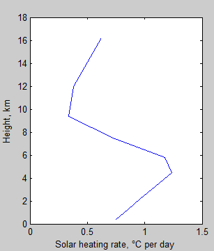
Figure 1
This is shown in °C/day but is easily converted to W/m² by dividing by 86,400 (number of seconds in a day) and multiplying by the heat capacity of that layer of the atmosphere. Each of the atmospheric layers in the model have roughly the same number of molecules so the graph of W/m² absorbed in a given layer looks quite similar in shape.
I introduced this solar heating partly because the old model had bad accounting at the top of atmosphere, where solar absorption just (magically) kept the stratosphere isothermal (the same temperature). That constraint is now gone in this update of the model.
Here is a model run:
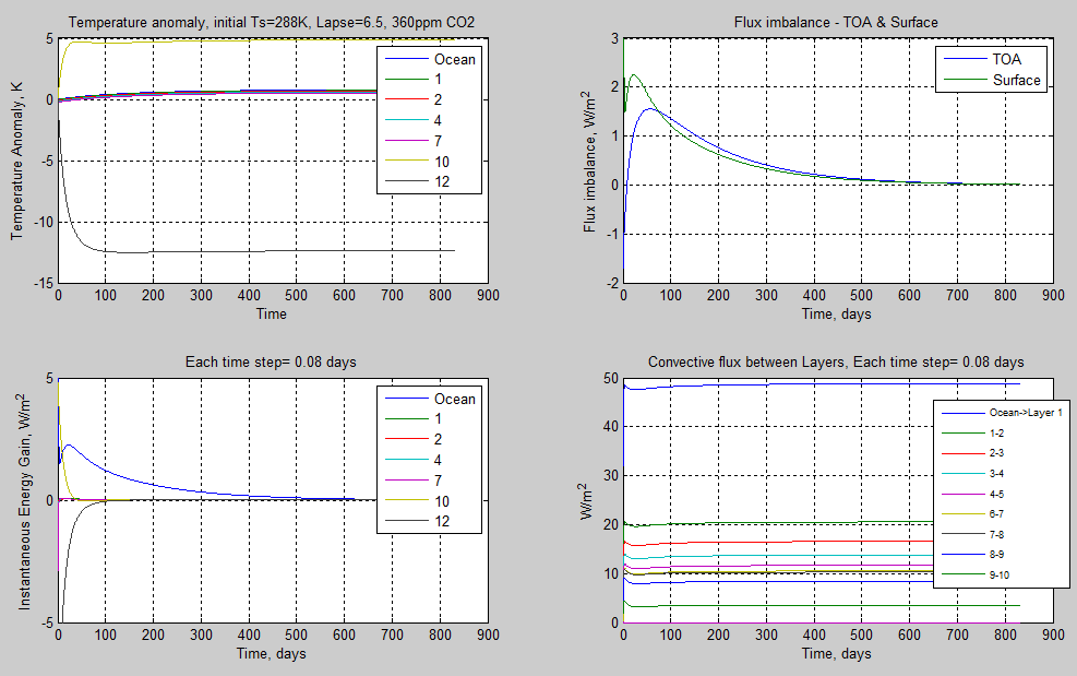
Figure 2 – Click to expand
What’s going on here? Well, let’s first take a look at the energy balance at the surface and for the whole planet (TOA):
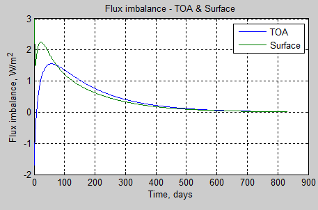
Figure 3 – Positive downward (so positive flux imbalance at TOA means the planet is heating up)
The starting point for this model was an ocean temperature of 288K and a lapse rate of 6.5 K/km, up to a tropopause of 200 hPa with an isothermal stratosphere. The solar radiation absorbed by the climate was 242 W/m², with about 100 W/m² absorbed in the atmosphere and the balance absorbed by the surface.
Each time step was 2 hours, and the model was run for 800 days (10,000 time steps).
Why is the model out of balance to begin with?
There’s no reason it should be in balance. I’ve simply prescribed a surface temperature and an atmospheric temperature profile and humidity and CO2 concentration. Why should that happen to be the steady state condition for the solar absorbed radiation of 242 W/m² with 100 W/m² absorbed in the atmosphere?
[Update Jan 22nd – A good point added from Pekka: “It’s perhaps not clear enough to every reader that this thread is describing what happens when the starting point is an initial state that you happened to choose rather than a state that the system could have reached at different external conditions. Thus the Figure 4 tells what happens initially for this specific case rather than values somehow applicable to the real atmosphere.”]
So the model works by energy accounting in each time step for each layer in the model. Energy cannot be created or destroyed. Radiation emitted and absorbed is calculated by the relevant equations (already explained). Convection moves heat if the atmosphere above is too cold (see Potential Temperature and Density, Stability and Motion in Fluids). Energy retained increases the temperature of the layer. Energy lost reduces the temperature of the layer.
Let’s consider the surface. On timestep 1 the surface is radiating 376 W/m² (note 1). All of the surface fluxes are shown (in W/m²) in the diagram:
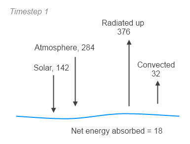
Figure 4
The net is 18 W/m² and so the “ocean” absorbs this energy which means it heats up. In 2 hours (one timestep) this comes to 129 kJ/m² and as the “ocean” in this model is just 10m deep (to allow quicker progress to any equilibrium) this equates to a temperature increase of 0.0031 °C.
If the net heat absorbed is 18 W/m² why doesn’t figure 3 show that? Ok, let’s zoom into the first month of figure 3 and we can see it clearly:
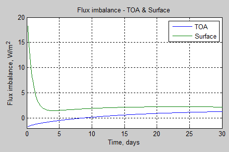
Figure 5
How did the convective flux get calculated? Why isn’t it higher?
The model calculates all the radiative fluxes up and down through each layer, works out the absorbed energy and the resulting temperature increase. Then it checks between each layer to see if the lapse rate is exceeded (see Temperature Profile in the Atmosphere – The Lapse Rate). This means the atmosphere would be unstable, resulting in convection.
The model then calculates the transfer of heat which would satisfy the lapse rate – the layer below loses X Joules, the layer above gains X Joules and new temperatures are calculated based on their respective heat capacities. This is what the model calculates and then adjusts temperatures, logs the convective heat moved and adjusts the energy change in each layer for that timestep.
The graph below zooms in on the first 30 days of the bottom right graph in figure 2:
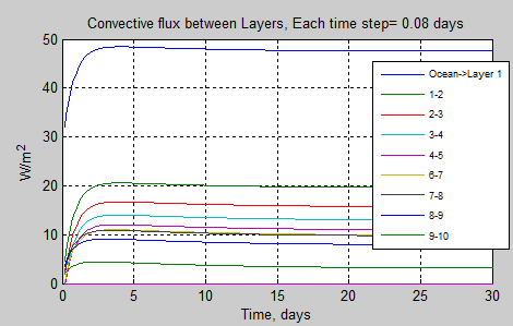
Figure 6
So convection in this particular instance isn’t any higher at the start simply because of the respective temperatures. Then the first atmospheric layer starts cooling via radiation (it loses more heat via radiation than it gains via solar heating) and this means that convection increases from the surface with each timestep – until a more steady condition is reached.
Now a key point is that the surface imbalance changes over time – which we see in figure 3.
Now there’s no magic “model driver” that makes this happen. It’s just basic heat transfer laws. The model just reflects, in a simplistic way, how heat is transferred between an ocean, an atmosphere and space.
Now let’s look at the TOA balance – look back at figures 3 and 5. This is the balance for the whole climate. What might be interesting is to see that the climate is initially out of balance – losing heat.
But why doesn’t the cooling of the climate mean that the imbalance just reduces until a steady state is reached? How is it possible for the climate to start heating at day 10 and peak somewhere around day 50 and then gradually reduce?
This is very typical of complex dynamic scenarios. Readers familiar with dynamic heat transfer (and any kind of dynamic physics/chemistry/engineering problems) will have seen these kind of graphs before – overshoot, decay to equilibrium.
What is completely unsurprising though is that the ocean and atmosphere end up in a steady state where cooling to space matches solar absorption – that is, the balance at TOA is ultimately zero.
Here’s a summary of the energy change, in kJ per timestep of 2 hours, of ocean, energy and TOA:
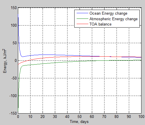
Figure 7
In the first few days the ocean and atmosphere are very much out of balance and so a big “reshuffle” of energy takes place where the ocean absorbs energy and the atmosphere loses energy until they are in much closer balance. Then there is a gradual cooling of the system (primarily via ocean cooling) which eventually leads to an overall TOA balance – which can be seen in figure 2.
In a subsequent article we will take this steady state condition, then increase the CO2 concentration and see what happens.
Conclusion
We’ve seen via one specific example how heat transfer, via radiation and convection, lead to a new equilibrium condition. This can include some oscillation on the way to equilibrium.
This particular case has no claim to be the “definitive median atmospheric condition”. It’s just a sample atmosphere that wasn’t in perfect balance for its conditions.
Many people have conceptual models of how heat moves in the atmosphere and often these mental models are wrong. The purpose of this article is to illustrate how the basic heat transfer mechanisms work. As we can see with this simple example, it would be surprising to get the right answer about dynamic and final temperatures from some hand-waving arguments.
If you have questions please ask. We can examine the energy transfer from many different perspectives.
Some Model Specifics
This update to the model has removed the constraint of keeping the stratosphere isothermal (see note 2).
Instead solar radiation is absorbed in the atmosphere according to the standard heating curves, for example, those found in Petty 2006 p.315:
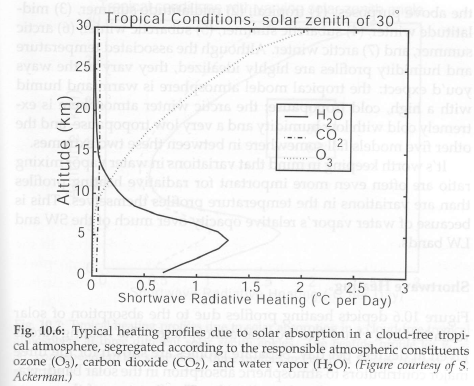
From Grant Petty (2006)
Figure 8
The stratosphere is not well modeled because the higher levels of the stratosphere are not included. These absorb most of the solar radiation via O2 & O3 and consequently keep the lower levels warmer than the equilibrium reached in this model.
This model had 12 layers, with the TOA at 20 hPa (most previous models had 10 going up to 50 hPa) – the reason for going higher was just curiosity about the resulting temperature profile.
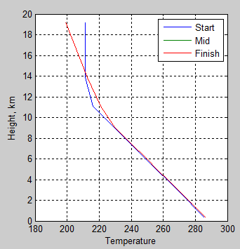
Figure 9
Clearly the solar absorption in the atmosphere should be calculated via the absorption characteristics of the various molecules but this will take some work, and the current model is just an interesting starting point (or resting place depending on my interest level in this aspect of the model). The main flaw in the current approach is that increasing water vapor in the lower atmosphere should increase heating via solar radiation but the model has a static absorption profile shown in figure 1. The main advantage is that it is a lot more accurate than having zero atmospheric absorption.
The convective accounting is also a little challenging. The problem is first that to calculate a convective adjustment we can’t just change layer 2 temperature to make it layer 1 temperature + lapse rate x height. Because after we work that out we have to move the right amount of heat from layer 1 to layer 2 to make layer 2 heat up enough. This reduces layer 1 heat by an equal amount and reduces layer 1 temperature dependent on its heat capacity and the temperature difference is now incorrect. This first problem is easily solved with a formula (see note 3).
Quick people unlike myself will immediately realize that we have not solved the problem at all because when we now consider layer 2- layer 3, the result will move layer 2 temperature and now layer 1-layer 2 is incorrect.
A bigger simultaneous equation might do the trick, but I’m pretty sure that it would come unstuck without some careful thinking about layers where the actual lapse rate in a given time step is less than the prescribed lapse rate. A quick solution was to do multiple loops (iterate towards a solution) and check the lapse rates via a graph and some printing out. Matlab is truly the friend of the mathematically lazy.
There are some checks and balances in my coding. Each time step the model calculates the difference between the TOA balance and the energy absorbed in all layers of the model. This should be zero otherwise I have not implemented the first law of thermodynamics. In this model run the maximum absolute error in any time step was 3 nJ/m² – or less than 4 pW/m². This is just rounding errors in the maths.
The model currently is tasked with printing an error message if ever more than 1J/m² goes missing in a time step.
The Matlab function returns the temperature profiles vs time, energy changes vs time for each layer, convective energy vs time for each layer, along with surface balance, TOA balance and lots of other parameters. The energy vs time graphs in figure 2 are shown as W/m² so they can be related to other fluxes, but they are stored as Joules per m² – it’s just difficult to consider whether 1.67 x 10⁵ J/m² is the kind of value we are expecting or not – and of course the (Joules) numbers change as the time step is adjusted.
Related Articles
Part One – some background and basics
Part Two – some early results from a model with absorption and emission from basic physics and the HITRAN database
Part Three – Average Height of Emission – the complex subject of where the TOA radiation originated from, what is the “Average Height of Emission” and other questions
Part Four – Water Vapor – results of surface (downward) radiation and upward radiation at TOA as water vapor is changed
Part Five – The Code – code can be downloaded, includes some notes on each release
Part Six – Technical on Line Shapes – absorption lines get thineer as we move up through the atmosphere..
Part Seven – CO2 increases – changes to TOA in flux and spectrum as CO2 concentration is increased
Part Eight – CO2 Under Pressure – how the line width reduces (as we go up through the atmosphere) and what impact that has on CO2 increases
Part Ten – “Back Radiation” – calculations and expectations for surface radiation as CO2 is increased
Part Eleven – Stratospheric Cooling – why the stratosphere is expected to cool as CO2 increases
Part Twelve – Heating Rates – heating rate (‘C/day) for various levels in the atmosphere – especially useful for comparisons with other models.
References
The data used to create these graphs comes from the HITRAN database.
The HITRAN 2008 molecular spectroscopic database, by L.S. Rothman et al, Journal of Quantitative Spectroscopy & Radiative Transfer (2009)
The HITRAN 2004 molecular spectroscopic database, by L.S. Rothman et al., Journal of Quantitative Spectroscopy & Radiative Transfer (2005)
Notes
Note 1: The emission of thermal radiation by a surface at 288K with an emissivity of 1.0 is 390 W/m². This is across all wavelengths. The model looks at the range of wavenumbers 200 – 2500 cm-1 (equates to 4-50 μm) to ease up the calculation effort required. Across this range the emission is 376 W/m².
Note 2: This was partly to avoid what would look like confusing energy accounting, where solar absorption = the amount prescribed in the model + what we find necessary to keep the stratosphere isothermal.
Note 3: If T1 and T2 are the unadjusted temperatures (found via radiative energy movement), and T1′ and T2′ are the temperatures that should result from lapse rate Γ and height difference z, then:
Convective heat, CE = [(T1-T2) – zΓ]/(1/Cp1 + 1/Cp2)
and then T2′ = T2 + CE/Cp2, T1′ = T1 – CE/Cp1


For future reference for me, the model run above was created via this command:
[ vt tau fluxu fluxd ztropo z dz p rho mixh2o zb pb Tb rhob …
Tinit T Ts dE dEs dCE radu radd emitu sheat surfe TOAe TOAf TOAtr alr]…
=HITRAN_0_10_1(1, 13, [1 2], [0 360e-6], [1 1], 9.2e4, .8, .4, 1, 1, …
288, 6.5, 6.5, 2e4, 2e3, 10, 242, 3600*2, 10000,1);
There are often questions about how heat capacity changes the results.
In simple cases increasing the heat capacity only lengthens the time to equilibrium – but the same equilibrium. So the equilibrium condition is identical, but the dynamic condition is different.
In complex cases, well, it’s more complex. But let’s understand the simple stuff first.
Here is the exact same run, but with the ocean depth set to 30m instead of 10m. The top can be compared with figure 3 and the bottom with figure 5 in the article:
SoD,
You could perhaps have explained in a little more detail the reason for the initial overshooting in the TOA flux imbalance. That occurs because the initial state it out of balance in many different ways. The reason for the initial negative value is the high temperature of the uppermost layer. That has a much stronger effect than the lower than equilibrium values of the ocean and lower part of the atmosphere.
The most rapid significant change that occurs in your calculation is the drop in the temperature of the uppermost layer. That pushes the imbalance up. The other temperatures adjust much more slowly with a pace determined largely by the ocean heat capacity. This adjustment leads to the slow approach towards zero imbalance.
What we see is thus a consequence of two factors:
– the presence of different time scales, because the ocean heat capacity is much larger than that of any single layer (and also larger than that of the whole atmosphere)
– the large, and opposite in sign, deviation from the equilibrium value of the initial temperature of the uppermost layer.
Sod,
I have had some argumentation with DeWitt in another tread and the nature of stratosphere came up in that discussion. That brought to my mind that your latest model could provide some help in understanding what the Earth atmosphere would do without solar heating. For that purpose I modified the model to allow keeping the surface temperature fixed at 288 K, while letting the atmosphere settle to balance as in your calculation. (I made those lines conditional, which modified the ocean temperature. Then I made that condition as well as the solar heating false.)
The result that I got is a tropopause at 10 km and a lapse rate around 2.8 K/km in the stratosphere. Thus the stratosphere turned out to have a temperature that falls with altitude rather than is constant as it is in the textbook theory of optically thin atmosphere. I did my calculation with 30 layers and minimum pressure of 20 hPa. Otherwise the parameters were the same you list in the first comment of this thread.
What do you think about your models applicability to such a calculation.
There was a mixup between two runs that I made. Actually I got those values for the tropopause and lapse rate when the model was essentially the same you have used. With the modified model the tropopause was raised to about 14 km while my minimum pressure was 10 hPa to cover better the high altitudes.
Pekka,
How did you define the tropopause? I think there are 3 definitions that can be used.
Pekka,
I think it’s a start, but once we get into the middle of the stratosphere the Voigt profile needs to be used, otherwise the atmosphere will be too optically thin. So with the current model the results can be questioned.
However, I think it’s worth pursuing because I have a lot of questions – like why the stratosphere cools with increasing CO2. Being able to investigate how radiative energy moves between layers and the impact of turning on and off different physics is quite fascinating.
SoD,
The definition that I have for stratosphere is the stratified atmosphere above troposphere up to the next level where the nature of the atmosphere changes. In a simple model case we have only troposphere and stratosphere. Tropopause is where regular convection stops; in simple models that’s the only convection we have.
The issue of optical depth and its relationship with linewidths is a bit more complex. The thin atmosphere would satisfy the assumptions of optically thin atmosphere much faster, it the lines were broad, not when the get narrower, because the theory presented in Pierrehumbert’s book requires that the atmosphere is thin on all important wavelengths, not on the average.
The narrowing of the lines is probably the main reason for the cooling of the upper stratosphere in your model as the radiation from below stays blocked at the optically active frequencies all the way to very high altitudes. Thus the effect of including Doppler broadening would ultimately lead to smaller lapse rate and less cooling at high altitudes.
One change to your way of handling layer depths should be made to study properly stratosphere. The stratospheric layers should not have equal mass but allowed to have progressively less and less mass to get more layers to stratosphere and through that more accurate results. I’ll try that soon.
It seems that adding the Voigt profile makes very little difference for IR as long as the pressure is 1 hPa or more, i.e. up to an altitude of around 50 km. At that altitude it increases the width of the main CO2 lines by about 50% influencing more the main peak than the tails. It’s more important for visible and UV, because the doppler broadening is proportional to the frequency. Very roughly the doppler linewidth is one millionth of the frequency at temperatures of troposphere and stratosphere.
I made an experiment by broadening the lines keeping the Lorentz lineshape. The results changed very little, probably less than the uncertainty in the model due to the limited number of frequencies as long as dv is not very small.
I did an improved calculation with about 20 layers in the stratosphere up to an altitude of about 45 km (pressure 1 hPa).
Here are the levels used in calculation, teperature profile, and lapse rate.
The tropopause is seen very clearly in the lapse rate. The increase of the lapse rate at highest altitudes is most probably due to the cutoff altitude of the calculation, but I haven’t tried to check that.
Here the Doppler broadening would influence the results and probably reduce the lapse rate in the stratosphere as the stratosphere would be heated more efficiently by radiation that’s not in the center of the narrow peaks whose upwards incoming radiation continues to be dominated by the nearest layer underneath.
The uppermost layer has the optical depth of 300 for one frequency of the 15µm band and 1 for another. Only two more exceed 0.1. With more broadening the maximum value would almost certainly be significantly lower, but the neighboring frequencies would get correspondingly stronger. A more uniform spectrum would lead towards the behavior of an optically thin atmosphere.
The calculation were done with the frequency step of 1 1/cm. That does certainly make the calculation inaccurate as the narrow lines are sampled very poorly with such a grid.
Pekka,
The lapse rate graph does not look very much like the derivative of the temperature graph. I suspect that what looks like a break point in the lapse rate graph is an artifact. Remove the break point and it’s not at all clear that there is a tropopause because there is never an inversion layer. Sure, potential temperature increases with altitude, but it does that in the troposphere in the real world too.
A small increase in lapse rate at high altitudes should be expected as the warming is caused by absorption of LW radiation by ozone. But that goes away at higher altitude. According to the graph in Petty, warming by ozone is at a maximum between ~23-28 km and then declines fairly rapidly. Above 30 km, ozone contributes to cooling to space.
I seriously doubt your model is correct, though. Above 15 km, there is net cooling to space from CO2 that overwhelms the warming from ozone. The lapse rate should be increasing, not decreasing. I suspect your line shape isn’t correct and you’re getting too much absorption of surface LW emission.
DeWitt,
I’m sure it’s not an artifact. It’s exactly what theory tells that we should expect. I have also varied many parameters and everything is very stable on qualitative level. Some variability is left in the quantitative values when the step in discretizing the frequency is varied.
There’s no ozone in this calculation, only H2O and CO2 and only CO2 is significant at high altitudes. There’s no absorption on solar radiation in the atmosphere, everything is based on IR only (plus convection up to the tropopause).
The basic mechanisms are the same as in the textbook case of optically thin atmosphere, but in that case the lapse rate drops directly to zero at tropopause while the drop is not that extreme here due to the large optical depth at the center of the strong CO2 lines.
Pekka,
Unless there is an actual inversion, there is no bar to weather. Think of a thundercloud. The typical anvil top is due to the inversion layer at the tropopause. Without that, the altitude the cloud reaches would be limited only by the available convective potential energy at the surface.
And you still haven’t explained why, if theory predicts an optically thin atmosphere will be stratified, the Martian atmosphere doesn’t have a stratosphere.
I’ll see your Pierrehumbert and raise you a Grant Petty:
A First Course in Atmospheric Radiation, Second Edition, page 70.
Your temperature profile is very much as Petty describes. The lapse rate never goes to zero, much less negative. There is no lid.
What I’d like to see is a plot of convective energy transfer vs. altitude.
Pekka,
The break point in the lapse rate profile is an artifact. It’s caused by using the kludge of a somewhat arbitrary fixed maximum lapse rate for calculating convective energy transfer. That same kludge is used in GCM’s and causes problems with them too.
DeWitt,
The thunderclouds present a strong example of what I mentioned as complexity related to weather phenomena. I had them in mind when I wrote my earlier message.
I wrote also already that the theory of optically thin atmospheres requires that the atmosphere is thin for every frequency separately. I did also explain that the Martian atmosphere is not at all like that.
I cannot explain Gran Petty, but I understand Pierrehumbert. When you brought the issue up I wanted to check myself that the line structure of the Earth atmosphere does not destroy the expectation. I’m pretty sure that my calculations using a slightly adapted version of SoD’s model did that in a reliable way.
One thing that I’m absolutely certain is that convection stops when lapse rate is less than the adiabatic one. That’s just basic theory that’s also presented in essentially every textbook. Strong convective currents can break the barrier for a while, but in general the upper limit of convection is given by the altitude where the lapse rates meet.
The break point is not a kludge. It’s true for a somewhat idealized model atmosphere. It’s true that the real atmosphere has smoother transitions, but that’s again largely due to weather phenomena and spatial variability that’s not even supposed to be caught in simple models. A large GCM aiming at a realistic description of the whole atmosphere should do better, but it’s not surprising that they may also turn out to be a bit idealized on this point.
I had in mind plotting the convective heat transfer rate as function of altitude, but that would have required a little extra code as it’s not stored in the present code (I think), but used indirectly. So far i haven’t plotted that.
DeWitt,
So if you have a layer of air with a potential temperature, θ1=330K and there is a layer 1km above with a potential temperature θ2=350K, what happens when a parcel is displaced quickly upward 1km from layer 1 to layer 2?
Does it sink back down, stay at layer 2, or keep rising?
[…] 2013/01/20: TSoD: Visualizing Atmospheric Radiation – Part Nine – Reaching Equilibrium […]
Why cooling in the stratosphere?
The convection begins when radiation lapse rate exceeds 6.5 K / km (Schwarzschild criterion). The scaling of the radiative transfer equation yields a greater height, where the Schwarzschild criterion actual. Characterized the troposphere thicker and the temperature difference between surface and tropopause increases. This increase in the temperature difference is to must be distributed between the surface temperature increase and decrease of the tropopause temperature – and so that the total radiation of the earth is constant.
Ebel,
If you mean why does increasing CO2 cause lower temperatures in the stratosphere, it’s simple. Increasing CO2 increases LW emissivity in the stratosphere while having almost no effect on SW absorptivity. The increased LW radiation to space causes an energy imbalance that is corrected by the temperature increasing less rapidly in the stratosphere with altitude. In other words, the stratosphere must cool to restore energy balance. If the CO2 concentration were high enough, the temperature wouldn’t increase with altitude at all.
Why cooling in the stratosphere?
Your statement is incorrect. With increasing CO2 concentration is the stratosphere colder and consequently decreases the LW emission and not increases (Planck formula). The elevated CO2 concentration increases the transport resistance and it is replenished less radiation energy transported and the stratosphere cools down so long, to have an decreases delivery and radiation to balance.
The reduced replenishment to the absorbed solar radiation produces a surplus of energy at the surface, which leads to the heating of the surface. The higher temperature of the surface, the radiation increases directly into space through the atmospheric wavelength window. The temperature increase is so long until the reduced solar radiation and the increased radiation by the wavelength window in the balance with the absorbed solar radiation. The CO2 concentration has always influence – even to the pure CO2 atmosphere like Venus.
One more thing: The Tropopausendruck on Venus is 0.4 mbar, the partial pressure of CO2 in the Erdtropopause about 0.13 mbar and rises by doubling the concentration to about 0.16 mbar.
At a higher concentration of CO2 the Erdtropopause moved toward Venustropopause – both in pressure and at the temperature.
SoD,
This might actually belong in an earlier part, but I’ll put it here because I’m basically lazy.
Using an arbitrary constant stable lapse rate that may be higher than the actual stable rate forces apparent convective energy transfer where none may actually be happening, or may be happening for reasons other than one-dimensional static stability, like three dimensional circulation. It’s basically a kludge to make the 1D model look like a standard model atmosphere.
DeWitt,
The lapse rate and vertical convection go always together. When air is rising or subsiding it’s temperature changes at a rate close to the adiabatic lapse rate. Conversely a lesser lapse rate than adiabatic prevents convection and a larger one induces convection.
There may be pressure gradients related to circulation that counteract (or strengthen) convection. These pressure effects are important, when the lapse rate does not deviate much from adiabatic.
Things are never as simple as an idealized small model, but the idealized small model can still capture the essential.
Additional:
Consider the fact that your humidity profile is constant with altitude above the boundary layer. This could not happen if there were only vertical convection from the surface. In that event, the RH would increase to 100% and the lapse rate would then be the saturated moist adiabat or pseudo-adiabat if precipitation is allowed. Constant RH means that vertical convection must be matched by downward flow of drier air which mixes at all levels. But that’s not in your model. It appears to me that your model assumes the conclusion that there is a tropopause and it’s at a particular altitude.
DeWitt,
It’s clear that the model has serious limitations. They are, however, not as essential at the top of troposphere and in lower stratosphere as they are in lower troposphere and higher stratosphere. The absolute moisture is low enough in upper troposphere and beyond to make the relative moisture unimportant. The value 6.5 K/km is probably too low for the upper troposphere. Thus the altitude of tropopause is perhaps too high, not too low.
There are other factors in the lower troposphere that may have an opposite effect, but even so my view is that the altitude is rather too high than too low. I’m not talking about tropical atmosphere where the moisture content is significantly higher, but about a typical atmosphere that the model is more likely to describe.
Pekka,
dCE(layer,timestep) captures the convective energy transfer. dC(1,:) is the transfer from ocean to layer 1, dCE(2,:) is from atmospheric layer 1-2, etc.
dCE is a subset of dE & dEs (ocean), i.e., you don’t need to add dCE to dE to get total energy. dE is total energy change each timestep in each layer (and dEs likewise for the ocean).
Fine. I didn’t spend much time for checking whether it’s available after the run.
Here is the convective flux as function of altitude.
As expected it decreases with altitude and is zero above the model tropopause.
Pekka,
130 W/m² convection from the surface! That’s impressive. Considering the humidity, that would all have to be sensible. But the temperature gradient between the surface and the atmosphere is nowhere near high enough to support that kind of heat transfer, not to mention the velocity of the upwards air flow required.
As I said: toy model.
Check what I wrote above.
The point is that simple models can describe some things, and the user must have an understanding on where that’s likely to occur and where not.
DeWitt,
This is correct. Regardless, actual potential temperature (which can be translated into lapse rate) determines the resistance of the atmosphere to convection.
That’s a question of whether we have the correct value. This is a different point from whether we have the right theory.
Increasing temperature in the stratosphere does prevent convection. But we don’t need that to prevent convection. Potential temperature is the important metric.
Basic dynamics says that if you provide a strong enough impulse you will get convection regardless of even an increasing temperature, let alone an even higher value of increasing potential temperature. That’s just about forces opposing motion.
Back to my question, if you displace a parcel from potential temperature θ1=330K to layer 2 where θ=350K does it keep rising or sink back down?
I think Grant Petty is using a different definition of the stratosphere. Suppose he’s not? He needs to explain atmospheric dynamics and why he thinks a decreasing temperature but increasing potential temperature still allows convection.
SoD,
Of course it sinks back down. But it does it somewhere else. Hydrostatic stability is only true over fairly large distance scales.
R. Caballero, p21.
Static vertical stability doesn’t prevent horizontal circulation. Horizontal circulation is driven by the surface temperature gradient. Yet another reason why a one-dimensional model is basically a toy.
Molecular conduction will never dominate eddy diffusion below 100km or so (the turbopause), at 1 g anyway. If it did, the molecular constituents of the atmosphere would no longer be well mixed. Eddy diffusion promotes energy conduction down a potential temperature gradient, forcing the gradient toward zero.
SoD,
You still have a magical element in your model: convective heat transfer from the surface. Exactly how do you get 48 W/m² to transfer from the surface to the atmosphere. Simple conduction won’t do it. You need a fairly large and stable temperature gradient for sensible heat transfer. That implies a cross wind to keep the diffusion layer thin. For latent heat transfer, you need a source of dry air to keep your humidity profile constant. Neither one seems to be in your model.
SoD, you say (referring to your Figure 4): “Let’s consider the surface. On timestep 1 the surface is radiating 376 W/m² (note 1).”
I find this a somewhat misleading statement. Or at least a bit halfway. Since the Earth’s surface is not a BB in a vacuum, the real (net energy/heat transferring) IR flux from the surface (to the atmosphere) in your model would be 376-284=92 W/m^2, not 376 W/m^2. In Figure 4 one might be confused into thinking that you liken the IR 284 W/m^2 coming down from the atmosphere, mainly heated by the surface, with the incoming SW solar flux, as if originating from a second heat source for the surface. In reality, that flux is part of the net energy loss flux from the surface. All it does is keeping the surface heat loss through thermal radiation down. I know you know this, and I know it doesn’t really change your conclusion, but wouldn’t it be better to just state this? IR from the atmosphere does not constitute a direct forcing on the surface. It’s an INdirect forcing, limiting its heat (net energy) loss by thermal radiation. The global surface of the Earth is always losing, never gaining, heat by thermal radiation. It is simply a matter of how great or small that loss is. This could be more clearly pointed out.
Thanks.
Kristian,
There’s nothing wrong with your way of thinking.
You can think of the 2-way radiative exchange as 1 net process or as 2 separate processes.
But regardless of the temperature of the atmosphere the surface radiates a given amount according to its temperature. Regardless of the temperature of the surface the atmosphere radiates a given amount according to its temperature. This is important to understand and many people (in the blog world) are confused about it.
Regardless of how you describe it in words, there is no actual difference. The only reason the earth is above the 3K microwave background temperature is because of the Sun heating it. So in this sense perhaps the arrow showing emission of thermal radiation from the earth is misleading, as people might think it is an independent heat source?
Understanding the individual fluxes and the net are both important.
SoD,
It’s perhaps not clear enough to every reader that this thread is describing what happens when the starting point is an initial state that you happened to choose rather than a state that the system could have reached at different external conditions. Thus the Figure 4 tells what happens initially for this specific case rather than values somehow applicable to the real atmosphere.
Pekka,
I think you are right and I updated the article with your comment.
SoD says: “Regardless of how you describe it in words, there is no actual difference. The only reason the earth is above the 3K microwave background temperature is because of the Sun heating it. So in this sense perhaps the arrow showing emission of thermal radiation from the earth is misleading, as people might think it is an independent heat source?”
That’s perfectly fine. I agree. BUT, if you want to determine HOW the positive imbalance (causing warming/net accumulation of energy) at TOA or Earth’s surface came to be, then you would have to sepate between the two – heat gain from the Sun and heat loss from the Earth. Then the specific terminology you use does become important. Because of the specific thermodynamic mechanisms for warming those terms represent.
Is the observed imbalance a result of increased heat gain or of reduced heat loss? The atmosphere reduces the heat loss. It does not increase the heat gain. Only the Sun does. Being an actual source of heat.
So, what if we observe increased total heat loss from the Earth’s surface and/or TOA during long-term global warming? That means the cause of the imbalance producing the net accumulation of energy in the system cannot be a heat loss reduction, i.e. atmospheric forcing. It will have to be an increase in heat gain, i.e. solar forcing. Will it not?
Kristian
Can you give an example?
Can you be specific on your terms because your statement is confusing (identify each term for surface balance and then which one or which combination you believe is the identifier).
If you observe heat loss from the Earth’s surface then there will be surface cooling. By definition. And the surface emission of thermal radiation at any time will only be due to the actual temperature (and emissivity) of the surface. So I can’t fathom your meaning.
If you want to separate out solar forcing there is an easy way – measure it via satellite.
SoD, you say: “Can you be specific on your terms because your statement is confusing (identify each term for surface balance and then which one or which combination you believe is the identifier).”
I’m not sure I see what’s so hard to understand.
I do realise that with a positive energy imbalance, there is only ONE real total heat flux and that is going down.
But what I’m getting at is the fact that this total heat flux CAN be split into a solar component and a terrestrial component, two net fluxes going in opposite directions.
The solar component is the warming one, the Sun being the heat source. The terrestrial component is the cooling one, the ventilation to avoid overheating.
So, Earth gains its heat from the net downward solar flux. At TOA or at the surface. At the same time it releases heat (from the surface to the atmosphere or from TOA to space). This is the net upward surface or TOA flux. At the surface this would constitute the sum of the global latent, sensible and net radiative energy fluxes, you know the ~165 W/m^2 that ideally balances the net incoming flux from the Sun.
And at the TOA, it would be OLR going OUT and SWin-SWout=SWnet going IN, you know the ~239 W/m^2 ideally going both ways.
We (I, at least) want to know which one of these two component net energy fluxes, the solar one or the terrestrial one, that has been responsible for the observed total positive energy imbalance (solar IN – terrestial OUT).
This is the background for my asking: “What if we observe that the total terrestrial net energy flux from the Earth’s surface and/or TOA has indeed increased during long-term global warming (let’s say the last 30 years)? Doesn’t that mean that the supposed warming mechanism of ‘the enhanced GHE’, restricting the Earth’s cooling rate (surface or TOA), simply could not have done the warming?”
Kristian,
To me it seems that it’s so far impossible to answer empirically your question.
The easiest part is the intensity of solar radiation in space. It’s being measured continuously and the measurements are accurate enough for this purpose. You can easily find data on total solar irradiance (TSI) from many sources.
The Earth albedo is the other factor for the net solar SW at TOA. Its not known as accurately. Measuring it from the satellites is difficult as the whole Earth area should be covered with a limited number of satellites and as also the short term temporal variability should be determined.
Similarly it’s difficult to measure accurately the total OLR at TOA. Again the satellites cannot do it accurately enough, more and better equipped satellites would be needed for accurate measurements both for OLR and for albedo determination.
At the surface accurate measurements of solar radiation are possible at individual points but covering the whole surface well enough is not practical.
In absence of accurate enough direct measurements the best we have are the analyses of the type of Trenberth, Fasullo, and Kiehl (2009): Earth’s Global Energy Budget. They combine evidence from a wide variety of sources and apply theoretical constraints in building their estimates. The can provide an useful overall picture, but they cannot really answer your question. The inaccuracies of their approach have been highlighted by some recent studies that tell about significant potential errors in their numbers. In particular the values obtained at surface are greatly uncertain.
Pekka,
SoD, in a January 2011 comment to his own post ‘Understanding Atmospheric Radiation and the “Greenhouse” Effect – Part Two’, stated:
“Imagine if all of the surface radiation was emitted unchanged at the top of atmosphere. (No “greenhouse” effect). Let’s say 450 W/m² emitted from the surface and, therefore, 450 W/m² emitted into space from TOA. Now we add a “greenhouse” gas and the radiation leaving from TOA = (e.g.) 440 W/m². The energy leaving the planet has reduced by 10 [->] 440 W/m². This means more heating of the planet, therefore, (by convention), a radiative forcing.
So it’s more about convention. If less energy leaves the planet, the planet must warm (at least in the short term). So a reduction in radiation leaving is an increase in radiative forcing.”
This, in place of a current answer on his part, like your response here (albeit tacitly and implicitly), seems to acknowledge the basic premise underlying my proposition.
Kristian,
So on the subject on whether or not solar radiation has increased or not, or is relevant or not – you don’t want to discuss it?
It’s irrelevant?
You claimed something about it – “So what would have caused the energy imbalance in this scenario? If not less energy OUT. There is only one alternative. More energy IN. From the Sun.” – this is now irrelevant?
I responded – “So this means that if the planet has warmed during this period it is not due to incident solar radiation.
And you spent several paragraphs on it including saying my comment was “..deductively invalid..”
Now you respond, on my request for clarification:
This presupposes I understand what your point is.
You have made claims about my understanding and motives. You have made claims I have tried to address.
Of course, at the end I ask you to actually answer your original points. If they were irrelevant why did you claim them?
Maybe along the way I am not sure what your argument is. This happens.
When I try to make sure I have understood your argument you claim that the point I am asking about – the point that you made, that you responded to, that you spent time on, accusing me of not being able to understand logic – that point was irrelevant.
This seems unfair.
My only method of understanding the multitude of people who arrive on this site with some new claim is to ask them to be specific. And to question each point. Frequently people claim I have quoted them out of context, avoided the subject, or been deceptive or misleading. Or antagonistic.
Everyone is convinced not only of their own absolute grasp of atmospheric physics, but also, of their absolute clarity in presenting their argument.
Only a small child or a golden retriever could possibly misunderstand the point.
Or someone deliberately trying to avoid the topic.
You can join these people. Of course, they have a completely different point from you. And probably a contradictory one.
If, on the other hand, you want to discuss and get to the bottom of the subject then you will need to take some time.
And if you have made a point and I ask about it, you will need to either say
– “ok, that actually wasn’t relevant”, or
– “I think you have misunderstood what I was trying to say there” or
– “here is why this is correct and I think you are wrong”
That’s one way. Or, say
– “you are being antagonistic”.
Up to you.
Again with the solar? This isn’t about the solar! Why this insistence of making this a solar issue? It is not. It is an OLR issue.
I apologize if you feel I’ve somehow insulted your intelligence. But read my answer again. I explain to you there why I find your conclusion and premise invalid. I explain there that when I say ‘more energi IN’ that means ‘relative to energy OUT’.
SoD, you say: “My only method of understanding the multitude of people who arrive on this site with some new claim is to ask them to be specific. And to question each point. Frequently people claim I have quoted them out of context, avoided the subject, or been deceptive or misleading. Or antagonistic.”
There is one easy way to avoid this.
What I normally do, and what I thought was customary to do, when faced with a ‘new’ argument or line of argument, is to wait and let the argument be laid out in full first so that I, with a skeptical mind, but in good faith, can thoroughly and objectively assess it from A to Z. If I start breaking up the flow of the argument presented right away, picking on details that I don’t understand or have issues with along the way, it will all come apart. Then the totality and the meat of the argument will be lost on me. And I will simply dissmiss it. Without even having made an effort to understand it. The actual argument.
Have you tried this approach?
In short: Focus lost.
[…] solar radiation at 242 W/m² with some absorbed in the stratosphere and troposphere as shown in figure 1 of Part Nine – Reaching Equilibrium […]
This is from Kristian
Pekka,
SoD, in a January 2011 comment to his own post ‘Understanding Atmospheric Radiation and the “Greenhouse” Effect – Part Two’, stated:
“Imagine if all of the surface radiation was emitted unchanged at the top of atmosphere. (No “greenhouse” effect). Let’s say 450 W/m² emitted from the surface and, therefore, 450 W/m² emitted into space from TOA. Now we add a “greenhouse” gas and the radiation leaving from TOA = (e.g.) 440 W/m². The energy leaving the planet has reduced by 10 [->] 440 W/m². This means more heating of the planet, therefore, (by convention), a radiative forcing.
So it’s more about convention. If less energy leaves the planet, the planet must warm (at least in the short term). So a reduction in radiation leaving is an increase in radiative forcing.”
This, in place of a current answer on his part, like your response here (albeit tacitly and implicitly), seems to acknowledge the basic premise underlying my proposition.
Yes, if less energy leaves the planet (OLR at TOA – terrestrial component) and the amount of energy entering the Earth system (solar component) remains unchanged over time, the planet must warm. And such a reduction in radiation leaving Earth is ‘by convention’ an increase in radiative (atmospheric) forcing. If this forcing keeps on strengthening, the warming will endure.
But if we DON’T observe less energy leaving the planet over an extended period of global warming, but rather the opposite – if it is observed instead to increase more or less in step with the rising surface temperatures, then what?
Then we have global warming which couldn’t possibly have been caused by less energy leaving the system – because more, not less, energy has been leaving the system during the warming. There is no way, then, that the atmosphere has been doing the work. The atmosphere has been doing its best to COOL the Earth, to keep the pace and to catch up with the imposed positive imbalance. How? By speeding up the global water cycle. Higher rates of evaporation and convection to spread the accumulated (mainly tropical) surface heat around the globe and to lift it ever more efficiently up and away from the surface towards TOA and space, warming the troposphere along the way.
So what would have caused the energy imbalance in this scenario? If not less energy OUT. There is only one alternative. More energy IN. From the Sun.
Pekka, I would like to see you build a case for OLR at TOA (as measured by satellites – e.g. ERBE-CERES, ISCCP FD, HIRS) not having increased as a function of general surface temperatures since at least the mid 80s, global evaporation/latent heat transfer from the surface of the Earth not having intensified significantly since the 70s and the temperature gradient between the global sea surface and the air layer directly above it not having become steeper since the end of the 70s.
If you can do all this, you would have shown that the Earth system has NOT managed to shed more of its incoming net energy (from the surface, through the TOA) as a result of/a response to higher surface temperatures. In line with the atmospheric warming mechanism – restricting heat loss to promote accumulation of heat.”
Thanks, SoD:)
Kristian,
The observing systems in place answer one question:
1. Incident solar radiation has not been observed to increase since 1979. (Pre-1979 nothing was in place).
So this means that if the planet has warmed during this period it is not due to incident solar radiation.
Let’s check you agree on this point? Theory and measurement – are we in agreement?
The observing systems in place can comment on TOA OLR for just over the last 10 years. This system is CERES.
Here is an output from CERES, and you can do it yourself in a few minutes..
The top graph is reflected solar, the bottom graph is incident solar.
It seems from your comments to date that you think something is obvious.
I’m often slow so please outline what exactly you think and why.
I’ll start the ball rolling:
– incident solar radiation has not increased
– there might be a slight trend in reflected solar radiation over an earlier longer time period- as outlined in The Earth’s Energy Budget – Part Four – Albedo
– from 2000 – 2012 there is some year to year variability in OLR but no clear trend; the year to year variability I hope to talk about in a later article
Over to you.
SoD,
Thanks for answering.
I’ll divide my reply into parts in order to make it a bit more manageable/readable.
Here goes …
First you state the following: “The observing systems in place answer one question: 1. Incident solar radiation has not been observed to increase since 1979. (Pre-1979 nothing was in place).”
Could you please provide the source on which you base this claim? I’m not necessarily saying I disagree, but it would be nice if you could present some documentation for it. What are these ‘observing systems’ that you speak of in this specific case? And what specifically do they show? Over the time period 1979-2012. Are there more sources than one? And do they all tell the same story?
From the statement above you then draw the following definite conclusion: “So this means that if the planet has warmed during this period it is not due to incident solar radiation.”
That’s quite a remarkable statement. And deductively invalid.
You very well know that the planet warms according to the total energy imbalance, not according to whether the heat input from the Sun (solar component, which is always positive) has been going up, down or stayed flat during the warming.
If the Earth system receives on average more net energy (IN) from the Sun than it manages to give off back (OUT) to space, then it will warm from the resulting positive energy imbalance. It doesn’t matter if Earth’s energy input from the Sun is decreasing in magnitude over time. As long as it’s greater than the planet’s total energy output, the warming will continue, albeit at a slower and slower pace, until the imbalance has finally been brought back to zero (assuming in this case the output stays unchanged).
This means it is not the change in incident solar we need to assess to find out what causes global warming. Global warming by the Sun can and will happen as long as the Earth system doesn’t adequately manage to vent out the constantly incoming heat. The Sun is our heat source after all and whatever it does it will always warm us. Its distinctive contribution will always be positive. Whether its absolute intensity goes up or down.
The atmosphere on the other hand can only make us warmer by restricting the natural cooling process (working parallelly with but in the opposite direction to the heating process) of the Earth system to space. That’s all it can do. It can never directly warm the surface of the Earth.
Therefore, to determine whether an ‘enhanced GHE’ is or is not the cause of the observed modern era global warming (over the last few decades), we must have look at the OUTGOING net flux. That is, OLR at TOA and/or the total net upward energy flux at the surface (the terrestrial component).
Here’s the bottom line: If OLR at TOA and/or the total net upward energy flux from the Earth’s surface is observed to INcrease rather than DEcrease during long term warming, then we KNOW that the atmosphere has not caused the warming. Why? Because the cooling process has strengthened rather than weakened, as a RESPONSE to the warming.
Solar warming:
direct heating of the surface –> cooling process responds
Atmospheric warming:
cooling process is restricted (decreases in strength) –> surface responds by warming up
You see the opposite courses of events …
Check out this:
http://klimaforskning.com/forum/index.php/topic,1148.msg21543.html#msg21543
Which brings me to your CERES plots.
If you recall, I clearly stated that the OLR at TOA cannot be observed to increase DURING WARMING, if the atmosphere is to be responsible for that same warming.
Well, there has been no global warming during the lifetime of the CERES satellites (Terra and Aqua).
So why would we expect to see any trend resolving the issue in the CERES OLR data? We wouldn’t.
But CERES wasn’t the first satellite project to measure OLR. And I think you know this, even though you stated the following: “The observing systems in place can comment on TOA OLR for just over the last 10 years.” Well, I already mentioned several other projects in my last post (to Pekka Pirilä).
But before we go there, let’s just agree on one thing. Looking at the CERES (anomaly) data, there is no question what controls OLR at TOA: 1) surface temperatures, 2) atmospheric temperature and humidity and 3) clouds, with 1) leading (basically ruling) 2) and 3). The ENSO process is the best way to show this.
Loeb et al. 2012:
Click to access art%253A10.1007%252Fs10712-012-9175-1.pdf
Susskind et al. 2012:
Click to access 20120012822_2012011737.pdf
With this is mind, let’s go back in time.
More later …
Kristian,
Are you playing a game?
Or just don’t understand how the first sentence linked to the second sentence?
I said “1. Incident solar radiation has not been observed to increase since 1979.”
And immediately following I said:
“So this means that if the planet has warmed during this period it is not due to incident solar radiation.”
You are absolutely correct that I have not been annoying pendantic in my response. I expected you to link the first sentence to the second sentence.
The word “so” was the clue.
And in any case it was in response to your previous comment which maybe you have forgotten, where you said:
This implied you believe increases in absorbed solar radiation are the cause of recent decadal warming. I took it to mean that anyway and perhaps every other reader would also think the same.
In any case I will rephrase my previous impossibly vague sentence and we can start again:
“So this means that if the planet has warmed during this period it is not due to an increase in incident solar radiation.”
I await your response.
Remember I asked “Let’s check you agree on this point? Theory and measurement – are we in agreement?“
And for the 30 years of history of incident solar radiation, see Here Comes the Sun.
Kristian,
Yes I do know this. But can they comment on trends in OLR prior to 2001?
Obviously you think they can, so please summarise the observing systems in place since 1979 with, for each:
– years in operation
– absolute accuracy
– accuracy in drift year to year
– spatial coverage
From these systems, what trends have been observed to what accuracy?
Kristian,
I’m told that on a Norwegian blog you (or someone appearing to be you) claim that I left your comment in moderation while letting other comments through, hinting at nefarious motives.
You can read Comments & Moderation to find out the story in moderation. In fact, WordPress puts stuff in moderation based on many reasons. One of them is the number of links in a comment. There are other reasons as well, use of certain names, theories and various reasons WordPress decides on like IP address because of other activities from that or similar IP addresses on other blogs.
Several of my comments have over the months ended up in moderation and one in trash bin. I have never found out why just those messages were selected for that treatment by WordPress. They didn’t differ in any obvious way from other comments that I wrote just before or just after from the same ip.
It’s a related phenomenon to what happens for the email that I receive. The junk mail filters make sometimes decisions that I cannot understand at all.
As we saw, the OLR at TOA tracks surface temperatures. Most of the global energy exchange occurs and the tightest convectional connection between surface and TOA exists within the tropical Walker/Hadley-cells, so this is where we would expect to (and do) see the closest fit and the largest amplitudes. As the CERES plots show, the global curve is more or less a slightly modified, dampened version of the tropical one – the tropical signal dominates (just as with global temperatures). This map tells us much of the story why:
http://ds.data.jma.go.jp/gmd/jra/atlas/eng/indexe_surface12.htm
The relatively close relationship between surface temperatures and TOA OLR found in CERES is confirmed further back in time by other satellite projects measuring OLR, so much so that it seems to be a robustly established relationship. These include ISCCP FD, ERBS/ERBE, HIRS and AVHRR (NOAA OLR Interpolated).
As you’re probably well aware, global (and tropical) temperatures haven’t gone up within the last several years. In fact, the last time the global surface mean temperature level made a jump was in the near aftermath of El Niño 1997/98. Before that the same thing happened in the immediate wake of El Niño 1986/87/88. And this general step-up only occured at these two specific instances. There has been no general increase in global temperatures outside these two upward shifts. Since 1979:
Three of the four satellite datasets mentioned above agree almost surprisingly well with one another. Furthermore, they all span different yet overlapping time periods. There’s a transitional gap between the end of the ERBS/ERBE data in 1999 and the beginning of the CERES data in 2000, but both HIRS and ISCCP FD have data that bridges that gap, making it fairly straightforward to merge ERBE with CERES. By all means, there is no guarantee here for full certainty about accuracy, absolute magnitudes and amplitudes. This isn’t necessarily the final truth. But it’s what we’ve got. These are the best data at hand. We cannot go back and do it again, measure it once more. It’s done. The numbers are in. And, most importantly, they seem to fit, they seem to make sense. They all seem to share a clear common pattern (the ‘pattern’ is what matters), the same pattern CERES shows: OLR tracks surface temperatures.
Earth’s surface temperatures have gone up. And so has OLR at TOA. In step with the temperatures. That is what the data shows. Even after a fair amount of downward adjustments.
Comparing HIRS and ERBE 1984-2000 (20N-20S):

Comparing ISCCP FD and ERBE 1985-2005 (20N-20S):

ISCCP FD global (as one can see, the same pattern as in the tropics, only with amplitudes subdued):

TOA fluxes (ISCCP FD vs. ERBS; note, these results are arrived at through different/independent methods):

Lee & Gruber et al. 2007 on HIRS:
Click to access Lee_et_al_07_HIRS_OLR_CDR.pdf
Wong & Wielicki et al. 2006 on ERBE/ERBS:
Click to access Wong-Wielicki-et-al-2006-J-Climate.pdf
Zhang et al. 2004 on ISCCP FD:
Click to access 2003JD004457.pdf
ISCCP FD and ERBE/ERBS 20N-20S vs. tropical temperatures (HadCRUT4):

(Note the downward adjustment in 2001 in the FD data. ISCCP explains: “[…] the sudden increase in upwelling LW flux in late 2001 may be exaggerated because it is associated with a spurious change of the atmospheric temperatures in the NOAA operational TOVS products that are used in the calculations.”)
ISCCP FD global vs. HadCRUT3gl:

(Note the slight upward adjustment in the FD data 1994-99 – this is consistent with ERBE/ERBS tracing higher (in the tropics) during this particular period and also with the surface temperatures. Also, the post 2001 data is adjusted down here like in the tropics.)
HIRS (and CERES from 2000) vs. HadCRUT3gl 1979-2012:

Finally, HIRS vs. NOAA OLR Interpolated (AVHRR), the fourth satellite dataset, riddled with problems such as uncorrected data inhomogeneities and satellite drift, but still displaying an overall pattern resembling the others over time:

Here you see some of the problems, and also a somewhat arbitrary attempt at correcting the series, making the long term evolution losing its general upward trend (which as it happens it shares with all the other datasets), which makes one think that the people behind the correction were more interested in esthetics (read: flatness/symmetry) than portraying reality as best they could:

Here’s the paper:
http://journals.ametsoc.org/doi/pdf/10.1175/2009JTECHA1366.1
Conclusion: OLR at TOA has gone up during the last ~3 decades of general warming (that is, temperatures only rose at two specific instances, as did OLR). No matter how one twists and turns, how much one would like to point to uncertainties in these data (despite the close match between different projects), one would have a pretty hard time finding in any of these datasets a gradual and general decrease in OLR during this time period. Or be it a flat trend, no increase whatsoever.
What does this mean? To the best of our knowledge today, based on the best available data at hand, there is no way restricted cooling of the Earth system (atmospheric forcing) has caused the positive global energy imbalance we’ve been seeing now for a while. The cooling processes have intensified in step with the surface warming. This directly counters the working mechanism for atmospherically induced warming. It simply does not work with enhanced cooling.
More on surface fluxes/energy balance later …
SoD,
Forget about the solar (heating) component (I explained why). This is about the terrestrial (cooling) component. That is the net flux relevant to the hypothesis of ‘the enhanced GHE’. If that net flux increases, there is no ‘enhanced GHE’, because the ‘enhanced GHE’ can only warm the surface by disallowing this flux to increase. It’s purely a theoretical construct, its real-world effect undetectable.
Kristian,
In response to your comments of:
1. February 2, 2013 at 2:33 pm, and
2. February 2, 2013 at 2:36 pm
I responded:
1. on February 3, 2013 at 1:55 am – incident solar radiation
2. on February 3, 2013 at 4:06 am – observing systems
Your long responses at February 3, 2013 at 10:58 am and February 3, 2013 at 11:03 am ignored both of the questions I asked.
Would you like to respond to them? By respond I mean specifically address the points that I made in response to the points you made.
This includes your claim “That’s quite a remarkable statement. And deductively invalid.” (= you didn’t read my comment?)
And your claim and “And I think you know this, even though you stated..” (= a claim of deception on my part?)
Alternatively, if you just want to post long comments without engaging with responses I make to your earlier comments I will choose whether or not to respond.
No doubt you can then claim on your own favorite blog that I am unable to respond to your impressive points. Up to you.
And in your long comment that didn’t address the specific responses I made I note that you made 2 points:
“..As we saw, the OLR at TOA tracks surface temperatures..” – do you think I don’t agree with this?
“..ISCCP FD have data that bridges that gap..” – do you know where ISCCP data comes from? Is it an observing system?
Engaging with people in a debate means engaging, not just writing very long comments with 10 points and when someone actually addresses one of them, writing another comment with another 10 points.
Especially when you have claimed that that person cannot understand basic premise logic on point 1 and been deceptive on point 2.
Some people call this the “gish gallop” approach to debate.
It isn’t debate.
Kristian,
The standard explanation is that the TOA imbalance has built up from the restriction in OLR. As long as the rate of warming is constant and absorbed solar is also constant, OLR must by identity also remain constant.
As increasing temperatures mean that more LWIR is emitted constant OLR means that the atmosphere has to resist stronger its release to space.
By the above a constant OLR is the expecation. A deviation from constancy by an amount that’s significantly less than the imbalance is allowed but changes that are larger that the imbalance would contradict the standard explanation.
Changes in the rate of warming of the surface and the atmosphere should also be taken into account in the comparison to improve its accuracy.
SoD,
It was never my intention to indicate any nefarious motives on your part. I simply reported what was going on here (our exchange) on my home forum. I even stated what you stated here, what your Comments section describes. Other commenters did hint at such motives, but I clearly emphasized that I trusted the procedure to be exactly as you explained.
You run a public blog here so I’m sure you acknowledge the fact that it will be and is commented on on other sites.
Regarding the specific case of allegedly claiming that you left my comment in moderation while letting other comments through is just stating fact. I posted two comments in relatively quick succession. The first one got right through, the other one was held up in moderation (even though you state that you don’t do moderation). That’s all I said, as background information to my posting that specific comment in moderation here on my home forum. I never said anything about other people’s comments being let through before mine. It was all about those two comments, both mine.
I see now that comments containing several links might be put on hold like this. If so, is this an automatic WordPress thing?
Ending up in moderation is an automatic decision by WordPress and largely out of control of the host of the site.
I told, how that has happened at two levels of severity to my comments, and I’m fully convinced that it all done automatically by WordPress.
Kristian on February 3, 2013 at 11:54 am:
That’s what I said. I don’t moderate.
WordPress has automatic moderation built in, some of the rules are from me, some of the rules are from WordPress. Some of the rules relate to how many links, specific phrases, etc. The WordPress rules are not explicit to me – I cannot see them. They just do stuff. This blog is hosted by WordPress so their automated rules apply.
You can tell that I don’t moderate because when you post most comments they just appear and it is only on occasion they say “..in moderation”.
Blogs which moderate as standard (i.e. every comment must be approved) will always say “..in moderation” for a period of time from a few minutes to many hours.
And just to conclude on moderation, of course I can put your name into my WordPress rules for moderation (I haven’t).
This means every comment by you will end up in the moderation queue and I can then decide whether to keep it waiting for 1 minute, 10 minutes or 10 hours.
But you will know, because every time you comment it will show up with “..in moderation”.
I found that some sites where I am not popular I start off commenting and it appears straight away, and then later, when I have annoyed the host, every time I comment it shows up with “..in moderation” and then many hours go by before the comment appears, sometimes snipped, sometimes never to appear.
SoD,
You say: “Your long responses at February 3, 2013 at 10:58 am and February 3, 2013 at 11:03 am ignored both of the questions I asked.
Would you like to respond to them? By respond I mean specifically address the points that I made in response to the points you made.”
Not really, because they’re of no relevance to what I’m trying to say here. YOU’RE not addressing what I’M saying, SoD. The actual argument. So why should I go along with your specific picking on irrelevant points which only detracts attention from the main issue?
You’ve adopted a rather antagonistic tone and frankly don’t seem very interested in following the argument at all. You asked me to build my case. But when I try to do that, you apparently don’t want to hear about it.
You accuse me of lengthy answers. What would you have me do? Explain this issue with a string of brief bywords?
Pekka Pirilä, you say: “The standard explanation is that the TOA imbalance has built up from the restriction in OLR.”
Yes, I know that this is ‘the standard explanation’. It’s just that the data from the real world doesn’t support it. It actually contradicts it.
SoD, you say: “Are you playing a game? Or just don’t understand how the first sentence linked to the second sentence? I said “1. Incident solar radiation has not been observed to increase since 1979.” And immediately following I said: “So this means that if the planet has warmed during this period it is not due to incident solar radiation.” You are absolutely correct that I have not been annoying pendantic in my response. I expected you to link the first sentence to the second sentence. The word “so” was the clue.”
To me it looks like you didn’t understand what I said. If you read it you will see that this is exactly what I did – I read your first sentence which has the baked-in assumption that incident solar radiation has to increase in strength to generate warming. Then you state quite bluntly, and based directly on this assumption, that since this hasn’t happened, then the Sun cannot be responsible for the warming we’ve seen. I then go on to explain why the basic premise/assumption behind your first statement isn’t valid. I did link your two statements. And I clearly pointed that out. Before explaining why I think the invalid premise also invalidates your conclusion.
SoD, you say: ““..As we saw, the OLR at TOA tracks surface temperatures..” – do you think I don’t agree with this?”
If you agree with this, why are we having this discussion at all? Surface temperatures have gone up. So has OLR at TOA. In step with them. That’s what we’d expect. And that’s what the data shows has been happening.
Pointing to DIRECT (solar) surface warming, not INDIRECT (atmospheric) surface warming.
So write down a few equations. Then we can not have any confusion.
I say d(TSI)/dt = 0, where TSI is decadally averaged incident solar radiation and t = time.
If you agree then it only takes one line from me and one word from you, and instead of me reading your comment and making the obvious (to me) conclusion we can both be in agreement.
Write down your energy balance equations, define your terms, and state which terms are changing or not changing, or the equation that links them.
Your words are unclear (to me). Equations can be used to reach clarity.
SoD, you say: ““..ISCCP FD have data that bridges that gap..” – do you know where ISCCP data comes from? Is it an observing system?”
So neither HIRS (which you left out of the sentence above) nor ISCCP FD are observing systems as far as you’re concerned …? Can you explain why? What about ERBS/ERBE? What about the match between the different methods? Same pattern. Have you looked at the graphs I’ve linked to? Temperature vs. OLR. From different sources. They all tell the same story.
All other things being equal OLR tracks surface temperature.
The factors that change this relationship are a) timescales and b) other atmospheric parameters.
As per my previous comment, write your equations down, define your terms.
Then I will know precisely what you are claiming.
But only do this if you want me to dig into specific points until we are clear where any disagreement lies.
Kristian,
You say that the data contradicts the constancy of OLR when the scale used in comparison is given by the imbalance.
You have listed a large number of datasets. What’s your conclusion on the rate of change of the global average OLR?
What are the limits of uncertainty for the global average OLR in your view?
How does the estimate compare with the value of 0.9 W/m^2 given by many as estimate for the present imbalance?
SoD,
What do you need equations for in this case? What equations?
This is really not a hard concept to grasp. And there’s absolutely no need for any maths to be able to do so. Or to agree on what the concept represents.
Frankly I don’t see how a clever guy like yourself can find this vague or hard to understand.
I’ve stated this now multiple times:
If OLR at TOA (terrestrial cooling) is observed to increase rather than decrease during long term global warming, then that means an ‘enhanced GHE’ (atmospheric forcing) cannot be responsible for the warming.
There really is no more to be said.
Adding to that: You can disagree with me on two points, SoD.
1) The basic premise, or
2) What the data shows.
That’s it.
Kristian,
And to add a comment separate to the TOA debate, the surface is much more difficult to comment on. My comment is that it is impossible to determine if there has or has not been a change of a few W/m2 in loss of energy from the surface over this period.
To determine the surface energy balance we have limited observation and most is calculated from models, with balancing terms to “close the budget” that have significant uncertainty.
Again, if you have a specific hypothesis about the change in surface energy budget over the last decade or more, please spell it out.
[…] Part Nine – Reaching Equilibrium – when we start from some arbitrary point, how the climate model brings us back to equilibrium (for that case), and how the energy moves through the system […]
[…] Part Nine – Reaching Equilibrium – when we start from some arbitrary point, how the climate model brings us back to equilibrium (for that case), and how the energy moves through the system […]
[…] Part Nine – Reaching Equilibrium – when we start from some arbitrary point, how the climate model brings us back to equilibrium (for that case), and how the energy moves through the system […]
[…] Part Nine – Reaching Equilibrium – when we start from some arbitrary point, how the climate model brings us back to equilibrium (for that case), and how the energy moves through the system […]
[…] Part Nine – Reaching Equilibrium – when we start from some arbitrary point, how the climate model brings us back to equilibrium (for that case), and how the energy moves through the system […]
[…] Part Nine – Reaching Equilibrium – when we start from some arbitrary point, how the climate model brings us back to equilibrium (for that case), and how the energy moves through the system […]
[…] Visualizing Atmospheric Radiation – Part Seven – CO2 increases Visualizing Atmospheric Radiation – Part Nine – Reaching Equilibrium […]
For people interested in datasets like ISCCP-FD and where they come from..
Calculation of radiative fluxes from the surface to top of atmosphere based on ISCCP and other global data sets: Refinements of the radiative transfer model and the input data Zhang et al, JGR 2004.
And then some useful detail, which might be interesting to some people:
What is ISCCP-FD?
– Just for people interested.
You seem very interested in ISCCP FD. Forgetting about ERBE and HIRS? And the good match between the three?
What’s wrong with these datasets in your opinion? You don’t like the data they’re presenting? If so, that’s fine. That’s your privilege. You don’t think they have been assessed? Bias adjusted/corrected? Verified/compared? Links to papers (like this one) are already attached.
Kristian on January 27, 2013 at 9:52 pm: “Pekka, I would like to see you build a case for OLR at TOA (as measured by satellites – e.g. ERBE-CERES, ISCCP FD, HIRS)”
Kristian on February 3, 2013 at 10:58 am: “The relatively close relationship between surface temperatures and TOA OLR found in CERES is confirmed further back in time by other satellite projects measuring OLR, so much so that it seems to be a robustly established relationship. These include ISCCP FD, ERBS/ERBE, HIRS and AVHRR (NOAA OLR Interpolated).”
Kristian on February 3, 2013 at 12:55 pm: “So neither HIRS (which you left out of the sentence above) nor ISCCP FD are observing systems as far as you’re concerned …? Can you explain why? ”
Obviously I was trying to divert attention away from your real point. Once again.
You know, the reason I brought it up was I had already asked you for your opinion on the datasets prior to CERES.
Clearly, someone – like yourself – who cites ISCCP FD as a dataset hasn’t done any research.
Just interested to see if you had any idea about the subject. Curiosity drives me in this blog.
When people understand their subject I would like to know more.
When they have no idea and get angry when asked for commentary on their chosen subject, I usually lose interest.
Just to correct a tedious point. Obviously ISCCP is a dataset. Someone has calculated stuff and put it into a file. I meant to write:
Bravo, SoD!
You seem to have finished the task of avoiding my actual argument by way of rather pouncing on irrelevant points and sticking to it.
You said: “Obviously I was trying to divert attention away from your real point. Once again.”
Yup. You’re exactly right.
You also said: “Just interested to see if you had any idea about the subject. Curiosity drives me in this blog. When people understand their subject I would like to know more. When they have no idea and get angry when asked for commentary on their chosen subject, I usually lose interest.”
Nice dismissal. No need to address what I’m actually pointing at after that one. HIRS, ERBE? Never heard of it. Close match with the ISCCP FD data, you say (from your quote: “After the necessary evaluation of the accuracy of these calculated fluxes [based on global, weather resolving measurements] against independent measurements, primarily by satellites at TOA […]”)? Nope. New to me.
And with that you can confidently go right back to championing your ‘LW radiation reigns supreme’ paradigm. Holding your head high. Having fought me off once and for all. ISCCP FD? Hah! Fail!
I thank you for your time. Or should I say apologies for taking it up?
In my comment of February 3, 2013 at 4:06 am I asked Kristian:
That’s because I thought that would be useful information. Knowing what datasets told us what might be a good starting point. And at that stage, it seemed to be part of whatever hypothesis Kristian had (which I wasn’t clear on as can be seen above).
On asking again for a response to this question, Kristian said:
The accuracy & time/spatial coverage of the pre-2001 data sources is not relevant. It detracts from the main issue, which is (February 3, 2013 at 1:34 pm):
And I can’t ask about what the data shows because it’s irrelevant while being the main point.
I apologize for being picky about irrelevant information like what constitutes a TOA flux measurement and the accuracy of said values, especially the accuracy of said long term values when they are outputs of a radiative transfer model.
Missing the point is my forte!
By the way, I haven’t studied the accuracy of the long term values from the various overlapping / non-overlapping TOA longwave and reflected shortwave flux measurements from 1979 to 2001 so if anyone else has a good handle on the subject I am curious to understand these numbers and their uncertainty better.
SoD, you say: “Knowing what datasets told us what might be a good starting point. And at that stage, it seemed to be part of whatever hypothesis Kristian had (which I wasn’t clear on as can be seen above).”
Really, SoD? Really? Not read my links, have you? Not seen my charts? Not interesting?
And you haven’t read all of those instances where I laid out my argument as clearly as possible?
“If OLR is observed to increase during long term global warming, then it means an ‘enhanced GHE’ (atmospheric forcing) cannot be the cause. Why? Because intensification of Earth’s cooling process during warming isn’t compatible with a warming mechanism needing to restrict that very cooling process to work.”
And,
“The best data at hand shows consistently that OLR has indeed increased in step with the warming. From the early 80s until today. During which time both atmospheric CO2 and water vapour has increased significantly.”
Your only response to this seems to be that the data cannot be trusted,
But where is your OLR data supporting your side of the argument, the idea of an ‘enhanced GHE’ doing the warming? Less total radiation leaving the Earth system in the long term.
BTW, increased OLR at TOA is also consistent with an increased net terrestrial energy flux from the surface of the Earth to the atmosphere during the warming (mainly achieved through a strengthened latent heat transfer flux). Confirmed also by a steepening of the temperature gradient between actual surface and air layer above it – greater heat transfer from surface to atmosphere.
But I guess you’re not interested in hearing more about it. Too many minor points in between to pick at.
Kristian,
I believe that the same satellite data shows a decrease in albedo over the same time scale, meaning that while TSI has remained constant, the amount of incoming radiation absorbed hasn’t. If the albedo measurements are correct, then SW absorption has increased. The important number, then, is not upwelling LW at the TOA alone, but the radiative balance of incoming SW absorbed – outgoing LW emitted. The problem here is that the precision and accuracy of the albedo and outgoing LW is not sufficient to close the balance to a precision and accuracy of less than 1 W/m², which is what would be necessary to either support or disprove atmospheric radiative transfer calculations.
And following DeWitt’s comment I did a check today with a representative atmosphere (US 1976), ran it to equilibrium with 336ppm CO2 (the value in 1979) and then stepped the value to 395 (the value in 2010).
The pseudo-radiative forcing (because I’m not yet calculating it correctly in that stratospheric adjustment isn’t taking place) was about 1 W/m2.
So, if CO2 suddenly increased from 336 ppm to 395ppm we should see a step reduction in OLR of 1 W/m2.
As CO2 increased gradually over the 30 years in question, if temperatures didn’t rise to compensate for this reduction we should see a gradual reduction in OLR of 1W/m2 over 30 years.
If temperatures did rise to compensate what we would see instead would be no trend.
In fact, the observing systems do not seem capable of measuring a 0.3 Wm-2 decade-1 trend, which is why I earlier asked for my attention-diverting value of accuracy of each satellite observing systems pre-CERES (absolute & drift) plus spatial coverage and periods in operation.
And in any case, as already noted, we wouldn’t expect an OLR trend of 0.3 Wm-2 decade-1 even if one could be measured.
What we see instead is year to year variability of a much larger magnitude, due to all of the factors which do drive OLR – and I will attempt to explain and illustrate this in the next article.
The heat equation is an important partial differential equation that describes the distribution of heat (or variation in temperature) in a given region over time. In some cases, exact solutions of the equation are available; in other cases the equation must be solved numerically using computational methods . For example, simplified climate models may use Newtonian cooling, instead of a full (and computationally expensive) radiation code, to maintain atmospheric temperatures.