In recent articles we have looked at rainfall and there is still more to discuss. This article changes tack to look at tropical cyclones, prompted by the recent US landfall of Harvey and Irma along with questions from readers about attribution and the future.
It might be surprising to find the following statement from leading climate scientists (Kevin Walsh and many co-authors in 2015):
At present, there is no climate theory that can predict the formation rate of tropical cyclones from the mean climate state.
The subject gets a little involved so let’s dig into a few papers. First from Gabriel Vecchi and some co-authors in 2008 in the journal Science. The paper is very brief and essentially raises one question – has the recent rise in total Atlantic cyclone intensity been a result of increases in absolute sea surface temperature (SST) or relative sea surface temperature:
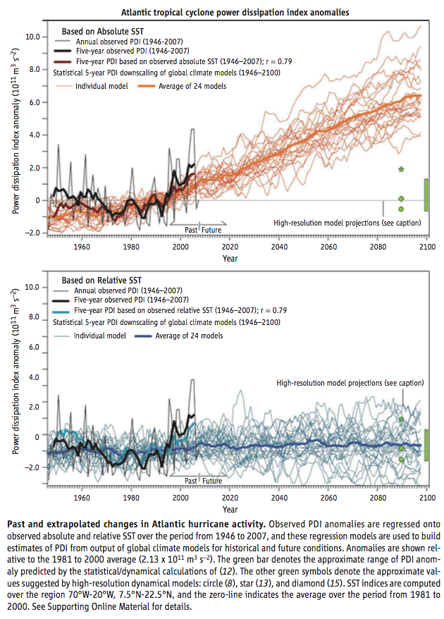
From Vecchi et al 2008
Figure 1
The top graph (above) shows a correlation of 0.79 between SST and PDI (power dissipation index). The bottom graph shows a correlation of 0.79 between relative SST (local sea surface temperature minus the average tropical sea surface temperature) and PDI.
With more CO2 in the atmosphere from burning fossil fuels we expect a warmer SST in the tropical Atlantic in 2100 than today. But we don’t expect the tropical Atlantic to warm faster than the tropics in general.
If cyclone intensity is dependent on local SST we expect more cyclones, or more powerful cyclones. If cyclone intensity is dependent on relative SST we expect no increase in cyclones. This is because climate models predict warmer SSTs in the future but not warmer Atlantic SSTs than the tropics. The paper also shows a few high resolution models – green symbols – sitting close to the zero change line.
Now predicting tropical cyclones with GCMs has a fundamental issue – the scale of a modern high resolution GCM is around 100km. But cyclone prediction requires a higher resolution due to their relatively small size.
Thomas Knutson and co-authors (including the great Isaac Held) produced a 2007 paper with an interesting method (of course, the idea is not at all new). They input actual meteorological data (i.e. real history from NCEP reanalysis) into a high resolution model which covered just the Atlantic region. Their aim was to see how well this model could reproduce tropical storms. There are some technicalities to the model – the output is constantly “nudged” back towards the actual climatology and out at the boundaries of the model we can’t expect good simulation results. The model resolution is 18km.
The main question addressed here is the following: Assuming one has essentially perfect knowledge of large-scale atmospheric conditions in the Atlantic over time, how well can one then simulate past variations in Atlantic hurricane activity using a dynamical model?
They comment that the cause of the recent (at that time) upswing in hurricane activity “remains unresolved”. (Of course, fast forward to 2016, prior to the recent two large landfall hurricanes, and the overall activity is at a 1970 low. In early 2018, this may be revised again..).
Two interesting graphs emerge. First an excellent match between model and observations for overall frequency year on year:
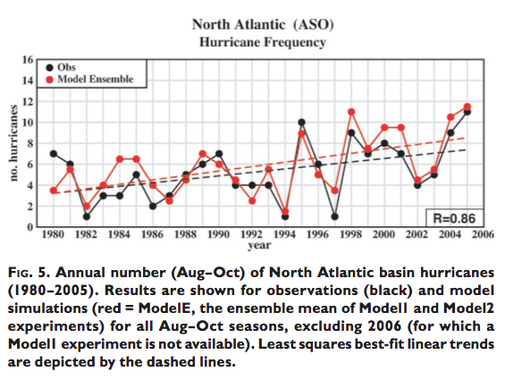
From Knutson et al 2007
Figure 2
Second, an inability to predict the most intense hurricanes. The black dots are observations, the red dots are simulations from the model. The vertical axis, a little difficult to read, is SLP, or sea level pressure:
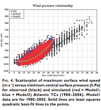
From Knutson et al 2007
Figure 3
These results are a common theme of many papers – inputting the historical climatological data into a model we can get some decent results on year to year variation in tropical cyclones. But models under-predict the most intense cyclones (hurricanes).
Here is Morris Bender and co-authors (including Thomas Knutson, Gabriel Vecchi – a frequent author or co-author in this genre, and of course Isaac Held) from 2010:
Some statistical analyses suggest a link between warmer Atlantic SSTs and increased hurricane activity, although other studies contend that the spatial structure of the SST change may be a more important control on tropical cyclone frequency and intensity. A few studies suggest that greenhouse warming has already produced a substantial rise in Atlantic tropical cyclone activity, but others question that conclusion.
This is a very typical introduction in papers on this topic. I note in passing this is a huge blow to the idea that climate scientists only ever introduce more certainty and alarm on the harm from future CO2 emissions. They don’t. However, it is also true that some climate scientists believe that recent events have been accentuated due to the last century of fossil fuel burning and these perspectives might be reported in the media. I try to ignore the media and that is my recommendation to readers on just about all subjects except essential ones like the weather and celebrity news.
This paper used a weather prediction model starting a few days before each storm to predict the outcome. If you understand the idea behind Knutson 2007 then this is just one step further – a few days prior to the emergence of an intense storm, input the actual climate data into a high resolution model and see how well the high res model predicts the observations. They also used projected future climates from CMIP3 models (note 1).
In the set of graphs below there are three points I want to highlight – and you probably need to click on the graph to enlarge it.
First, in graph B, “Zetac” is the model used by Knutson et al 2007, whereas GFDL is the weather prediction model getting better results in this paper – you can see that observations and the GFDL are pretty close in the maximum wind speed distribution. Second, the climate change predictions in E show that predictions of the future show an overall reduction in frequency of tropical storms, but an increase in the frequency of storms with the highest wind speeds – this is a common theme in papers from this genre. Third, in graph F, the results (from the weather prediction model) fed by different GCMs for future climate show quite different distributions. For example, the UKMO model produces a distribution of future wind speeds that is lower than current values.
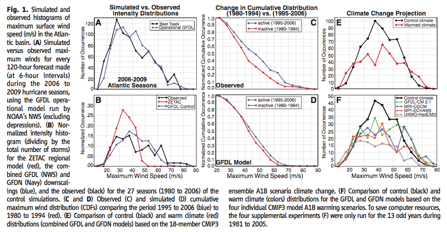
From Bender et al 2010
Figure 4 – Click to enlarge
In this graph (S3 from the Supplementary data) we see graphs of the difference between future projected climatologies and current climatologies for three relevant parameters for each of the four different models shown in graph F in the figure above:
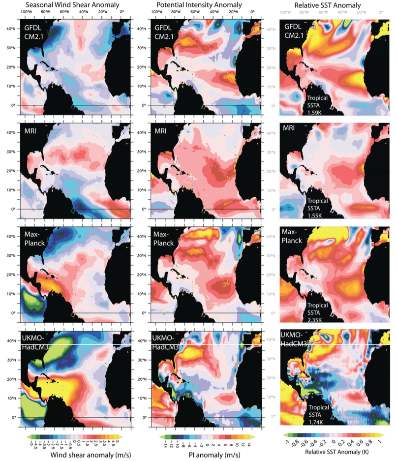
From Bender et al 2010
Figure 5 – Click to enlarge
This illustrates that different projected future climatologies, which all show increased SST in the Atlantic region, generate quite different hurricane intensities. The paper suggests that the reduction in wind shear in the UKMO model produces a lower frequency of higher intensity hurricanes.
Conclusion
This article illustrates that feeding higher resolution models with current data can generate realistic cyclone data in some aspects, but less so in other aspects. As we increase the model resolution we can get even better results – but this is dependent on inputting the correct climate data. As we look towards 2100 the questions are – How realistic is the future climate data? How does that affect projections of hurricane frequencies and intensities?
Articles in this Series
Impacts – II – GHG Emissions Projections: SRES and RCP
Impacts – III – Population in 2100
Impacts – IV – Temperature Projections and Probabilities
Impacts – V – Climate change is already causing worsening storms, floods and droughts
Impacts – VI – Sea Level Rise 1
Impacts – VII – Sea Level 2 – Uncertainty
Impacts – VIII – Sea level 3 – USA
Impacts – IX – Sea Level 4 – Sinking Megacities
Impacts – X – Sea Level Rise 5 – Bangladesh
References
Hurricanes and climate: the US CLIVAR working group on hurricanes, American Meteorological Society, Kevin Walsh et al (2015) – free paper
Whither Hurricane Activity? Gabriel A Vecchi, Kyle L Swanson & Brian J. Soden, Science (2008) – free paper
Simulation of the Recent Multidecadal Increase of Atlantic Hurricane Activity Using an 18-km-Grid Regional Model, Thomas Knutson et al, American Meteorological Society, (2007) – free paper
Modeled Impact of Anthropogenic Warming on the Frequency of Intense Atlantic Hurricanes, Morris A Bender et al, Science (2010) – free paper
Notes
Note 1: The scenario is A1B, which is similar to RCP6 – that is, an approximate doubling of CO2 by the end of the century. The simulations came from the CMIP3 suite of model results.


“With more CO2 in the atmosphere from burning fossil fuels we expect a warmer SST in the tropical Atlantic in 2100 than today”
The expectation that warming in sst is related to fossil fuel emissions is not supported by the data.
https://ssrn.com/abstract=3033001
This paper used a weather prediction model starting a few days before each storm to predict the outcome. input the actual climate data into a high resolution model and see how well the high res model predicts the observations.
Important to conceive this – climate models will never be able to predict the dynamic state of the weather which precedes tropical cyclone occurrence. And the “actual climate data” represents means, not the perturbed state which is what we’re interested in.
This exercise amounts to: “Well, if we could only predict the weather of the future, we’d know the weather of the future.”
But we can’t, don’t and won’t.
Turbulent Eddie,
The idea is to first of all find a way to get some accurate TC (tropical cyclone) metrics.
Perhaps with perfect data we can get an accurate representation – if so, the TC model is good and now we start to see what climate parameters affect TC formation and TC track (ie how many landfall in different areas). That is, we can use our accurate model with less accurate input data and find the sources of variation. Then develop a better theory about TC formation and TC strength. Possibly good results flow on that tell us, for example, that TC formation is dependent on relative SST, or on absolute SST, or has some other dependency. Then we can provide better data to people concerned about the future.
Perhaps with perfect data we fail to get an accurate representation – and if so, then we try higher resolution models, or attempt to identify the missing parameters that affect TC formation.
Science is often hard and as far as I can tell these people are doing it. Their approach makes sense given the current state of knowledge.
Dear Science of Doom,
The study you present is 9 to 10 years old. How did the ACE evolved between 2008 and 2016 ? It would have been interesting to compare this period with the 2008-2018 average predictions made in 2008 …
Ben, Hopefully we will come onto that, if a good recent study exists. First I try to explain the fundamentals.
Judith Curry wrote on Sept 8, 2017 …
For reference, the sea surface temperatures (ECMWF operational analysis) is shown below. Irma formed where SST was about 80F (26.5C).
In a matter of a few hours, Irma became a major hurricane. The surprising thing about this development into a major hurricane was that it developed over relatively cool waters in the Atlantic – 26.5C — the rule of thumb is 28.5C for a major hurricane (and that threshold has been inching higher in recent years). On 8/31, all the models were predicting a major hurricane to develop, with some hints of a Cat 5.
So why did Irma develop into a major hurricane? We can’t blame 26.5 C temperatures in the mid Atlantic on global warming.
The dynamical situation for Irma was unusually favorable. In particular, the wind shear was very weak.
Further, the circulation field (e.g. stretching deformation) was very favorable for spinning up this hurricane.
It’s complicated. If it wasn’t it would be less interesting and we likely would have figured it out long ago.
SOD wrote: “The top graph (above) shows a correlation of 0.79 between SST and PDI (power dissipation index). The bottom graph shows a correlation of 0.79 between relative SST (local sea surface temperature minus the average tropical sea surface temperature) and PDI.”
You don’t explain why the difference between local SST and global tropical SST should be important to hurricane intensity. Hurricanes aren’t powered by this difference in temperature.
I suspect a more fundament hypothesis is that mean global tropical SST’s determine the temperature near the top of the tropopause around the world – and therefore the temperature difference between local SST and the local top of the troposphere. Hurricanes are powered by this temperature difference. That difference is an important factor in calculating “potential intensity” (PI) of hurricanes. See your Figure 5.
The Wikipedia article on TC’s has a section on potential intensity. The square of the maximum potential wind speed varies with the temperature difference (T_s SST, T_o temperature of outflow near tropopause). Apparently AOGCMs indicate that this difference will increase in the future due to an increase in the height of the tropopause.
v_p^2 = \frac{C_k}{C_d}\frac{T_s – T_o}{T_o}\Delta k
https://en.wikipedia.org/wiki/Tropical_cyclone#Maximum_potential_intensity
That’s a good point, I didn’t explain and your explanation is what is put forward.
Here is Vecchi et al (2008), link in the article:
Reference 5 is Effect of remote sea surface temperature change on tropical cyclone potential intensity, Gabriel A. Vecchi & Brian J. Soden, Nature (2007):
Frank,
More comments on factors influencing TC formation:
TC-Permitting GCM Simulations of Hurricane Frequency Response to Sea Surface Temperature Anomalies Projected for the Late-Twenty-First Century, Ming Zhao & Isaac Held, Journal of Climate (2012):
Tropical cyclones in climate models, Suzana J Camargo and Allison A Wing, WIREs Clim Change (2016) – described as an advanced review:
– and “Emanuel and Nolan” = Emanuel K, Nolan DS. Tropical cyclone activity and the global climate system. In: Proceedings of 26th AMS Conference on Hurricanes and Tropical Meteorology
Of course there are problems.. Camargo & Wing continue:
SOD: Some additional info on the importance of the temperature difference for Potential Intensity (PI), which may be defined differently: SST and tropopause. Or T_s and T_o, where T_o is temperature of the air flowing outward from the top of the convective column of the hurricane. Or SST and cloud top temperature plus correction factor. As best I can tell, the fundamental reason we expect stronger hurricanes from climate change is an expectation that PI will increase due to a higher/colder tropopause or T_o.
IIRC, the Atlantic is the one basin where both the temperature difference has increased and hurricane intensity has increased. However, re-analysis products differ significantly about how much this temperature difference has changed over the decades. Year-to-year changes show the difference moves in parallel with observed hurricane ACE. Furthermore, the relevance of a basin average temperature difference between SST and tropopause is complicated by the fact that this difference isn’t uniform and it varies with the location of hurricane tracks, which move from year to year.
The formula I copied did not paste properly*
v_p^2 = [C_k/C_d]*[{T_s – T_o}/T_o]*[Delta k]
where T_s is the temperature of the sea surface, T_o is the temperature of the outflow, Delta k is the enthalpy difference between the surface and the overlying air ([J/kg]), and C_k and C_d are the surface exchange coefficients (dimensionless) of enthalpy and momentum, respectively.[30] The surface-air enthalpy difference is taken as Delta k = k_s – k, where k_s is the saturation enthalpy of air at sea surface temperature and sea-level pressure and k is the enthalpy of boundary layer air overlying the surface. Your more sophisticated formula for GPI uses V_pot (cubed), which I suspect that is the same v_p.
If I understand correctly, accumulated cyclone energy (ACE) is proportional to v^2 and power dissipation to v^3. Potential intensity (PI) is focused on the maximum work that can be done given the temperature difference and is proportional to velocity squared. It doesn’t depend on wind sheer and relative humidity, it appears to simply be potential work that can be extracted from the temperature difference. Your formula appears to try to predict how other factors will modulate simple PI. Since it uses velocity cubed, it may be a measure of power, rather than energy.
S-S Hurricane category varies with wind speed, ACE with wind speed squared, and power dissipation with wind speed cubed. A 10% increase in wind speed, becomes a 20% increase in ACE and a 30% increase in power dissipation. A 10% change in wind speed is about 1/2 of a category change.
Good point – what happens to To?
In the mean, GCMs predict a Hot Spot, which means To increases more, much more, than Ts.
So, Ts-To DECREASEs, and so max intensity decreases.
Hurricanes are discrete, not climatological means, of course, but I have a difficult time getting to any other conclusion, assuming the modeled hot spot occurred ( which hasn’t happened, of course ), that hurricane intensity should decrease.
TE: I presume you are referring to the predicted decrease in lapse rate, which results in more warming in the upper tropical troposphere than at the surface. This would reduce potential intensity (PI). However, if the tropopause rises and the outflow from hurricanes occurs at a higher altitude, T_o can still be lower.
In the online version of MODTRAN, In the tropics, the tropopause is 195 K at 17 km, 105 K colder than the surface. In midlatitude summer, the tropopause is 216 K at 13-17 km, 78 K colder than the surface. So the tropical surface is 6 K warmer, but the temperature difference (that controls potential intensity) is 27 K.
If tropical SSTs rose 3 K due to climate change and the hot spot rose 50% more (4.5 K), a 1 km increase in the height of the tropopause (-6.5 K) means the outflow temperature could decreases by 2 K or 1%. If the tropopause height increase is 2 km, the outflow temperature could decrease by 8.5 K. If the 6 K difference between midlatitude summer and tropical surface temperatures can raise the tropopause by 4 km
Frank,
You wrote “If tropical SSTs rose 3 K due to climate change and the hot spot rose 50% more (4.5 K), a 1 km increase in the height of the tropopause (-6.5 K) means the outflow temperature could decreases by 2 K or 1%. If the tropopause height increase is 2 km, the outflow temperature could decrease by 8.5 K.”
I don’t think it is the temperature difference that matters, it is the difference in potential temperature (or actually wet bulb potential temperature, which I am unclear on except that it is related to the wet adiabatic lapse rate). So Eddie might well be right that is the gradient that ultimately matters.
Mike M wrote: The standard formula for PI uses temperature not potential temperature, but your suggestion makes sense. If AOGCM’s are correct, the 2%/K increase in precipitation (not 7%/K) is caused by slowing the overturning of the atmosphere and a 1% increase in relative humidity over the ocean (suppressing the evaporation rate). So the future potential temperature difference would be larger than the future temperature difference.
… assuming you believe models describe convection, condensation and precipitation correctly. A decreasing lapse rate should weaken hurricanes, a higher outflow or tropopause should strengthen them, and higher relative humidity above the ocean surface should strengthen them. Models think the first factor is outweighed by the other two, but only to a modest extent.
I think most hurricanes don’t reach their maximum potential intensity. The factors that limit actual intensity or prevent organization could be more important than potential intensity.
Of course, this is all a bit speculative. The hot spot hasn’t occurred, at least for the satellite era. The hot spot is modeled to warm at a rate more than 2x the sea surface temperature. Not all of the out flow is at the tropopause. The suppression beneath the tropopause ( from sea surface to max hot spot, that hasn’t occurred ) is important. And the hot spot may be modeled because of erroneous convection parameterization ( which is guaranteed to be erroneous in some way or other because of it’s representation of dynamic discrete events ). That parameterization of convection also occurs with tropical cyclone modeling.
Here’s an interesting climatological feature of tropical cyclones, though:
Considering the mean paths of intensification, Atlantic cyclones intensify with mostly increasing SST. NE Pacific cyclones intensify with mostly decreasing SST.
Does this indicate that SST is not so important to tropical cyclone intensity?
Frank:
“If tropical SSTs rose 3 K due to climate change and the hot spot rose 50% more (4.5 K), a 1 km increase in the height of the tropopause (-6.5 K) means the outflow temperature could decreases by 2 K or 1%. If the tropopause height increase is 2 km, the outflow temperature could decrease by 8.5 K. If the 6 K difference between midlatitude summer and tropical surface temperatures can raise the tropopause by 4 km”
I was considering this a little more.
If one considers the NASA GISS A1B ensemble at 2100, the height of the 300mb level is modeled to increase by 100m, 30mb level by only a little more. So the tropopause height is modeled to rise by 0.1 kilometers or so.
Also, that rise is in part due to the Hot Spot forming. The Hot Spot is modeled to warm at twice the rate as the surface. So any potential decrease of stability from the surface to a rising tropopause is due to a large increase of stability for the 95% of the troposphere beneath.
Now, most of the tropics are always conditionally unstable ( meaning there’s plenty of buoyancy for parcels which get a critical lift ) most of the time. What this means is that tropical cyclones are not constrained by instability, but by low level convergence which realizes this instability.
Turbulent Eddie wrote: “The hot spot is modeled to warm at a rate more than 2x the sea surface temperature.”
I think that is strongly dependent on the models. Models that give large water vapor and lapse rate feedbacks get a strong hot spot, ones with weaker feedbacks get a weaker hot spot. But so far as I know, none of them do a good job on upper troposphere water vapor in the tropics. So I see no reason to believe any of them with respect to the hot spot.
Turbulent Eddie wrote: “Does this indicate that SST is not so important to tropical cyclone intensity?”
SST is a correlation not a cause. The cause seems to be conditional instability, which tends to be stronger when the sea surface is warmer. But that is not the only factor.
Turbulent Eddie wrote: “If one considers the NASA GISS A1B ensemble at 2100, the height of the 300mb level is modeled to increase by 100m, 30mb level by only a little more. So the tropopause height is modeled to rise by 0.1 kilometers or so.”
The tropopause is not defined by pressure, it is defined by the location of the temperature minimum.
Turbulent Eddie wrote: “Now, most of the tropics are always conditionally unstable ( meaning there’s plenty of buoyancy for parcels which get a critical lift ) most of the time. What this means is that tropical cyclones are not constrained by instability, but by low level convergence which realizes this instability.”
Isn’t that pretty much the same as saying that most of the tropics have sea surface temperatures of at least 26-27 C, so that is a necessary, but not sufficient, condition for cyclone formation?
Eddie wrote: “Also, that rise is in part due to the Hot Spot forming. The Hot Spot is modeled to warm at twice the rate as the surface. So any potential decrease of stability from the surface to a rising tropopause is due to a large increase of stability for the 95% of the troposphere beneath.”
I must confess to being confused by some aspects of this issue.
According to the conventional view, when tropical SSTs rise 3.0 K and the saturated adiabatic lapse rate falls due to increasing absolute humidity, then there must be more warming at the top of the troposphere than at the surface. Defenders of the hot spot insist that the tropics is dominated by a moist? or saturated? adiabatic lapse rate and therefore the apparent absence of a hot spot must be measurement error. However, relative humidity decreases with altitude, apparently even in the tropics. I presume this happens because of mixing between rising and descending parcels of air. So I don’t see how the tropical environmental lapse can depend on the saturated adiabatic lapse rate.
http://www.chanthaburi.buu.ac.th/~wirote/met/tropical/textbook_2nd_edition/navmenu.php_tab_6_page_2.4.0.htm
However, none of this means that the temperature difference between the surface and the tropopause must shrink. The location of the tropopause depends on the opacity of the upper atmosphere to thermal IR. At some altitude, the atmosphere becomes thin enough and dry enough that outgoing LWR is in equilibrium with incoming SWR at that altitude (minus reflection by the surface or by clouds). When such equilibrium exists, no convection and release of latent heat is needed to maintain a stable state. The location of the tropopause also depends on how much UV is being absorbed by ozone. I would enjoy reading a good post or paper explaining with the tropopause is where it is found today and why it will be higher (and colder?) in the future.
SOD, this reply is not for the current entry, but a previous one. Basically the issue I have with all responses of temperature increases over the last 150 years or so is the assumption that most of this rise is due to the increase in CO2. With that assumption, the models are adjusted to fit the rise with suitable assumptions in several parameters, which are limited in actual known effect. However, the temperature has clearly gone through several increases and drops of at least comparable magnitude even in the last 10,000 or so years, when CO2 could not be a major driver. Where is any evidence that in fact, the recent rise is due to CO2, and not mainly from other causes that also caused previous variation? I realize that human activity almost certainly has some effect, and likely cause the level to be somewhat higher that it would have been without humans, but attributing most of the recent rise seems a biased guess, due to the fact that human nature has a strong bias for events that happen over their lifetime. What would happen if models were fitted to a much smaller rise over natural variation, with say CO2 causing only 10% rise over natural levels (ie, subtract 90% of the present level of rise as a natural bias). Could the models fit this lower rise with suitable parameter choices?
Leonard,
You wrote: “What would happen if models were fitted to a much smaller rise over natural variation, with say CO2 causing only 10% rise over natural levels (ie, subtract 90% of the present level of rise as a natural bias). Could the models fit this lower rise with suitable parameter choices?”
I think the big problem with that is that we know that there is an anthropogenic forcing of about 2.3 W/m^2. If that is only 10% of the recent change, then there would have to be a natural change in forcing of about 21 W/m^2. There is nothing that seems to be able to do that. If you simply assumed a forcing of that size in a model, then you presumably could adjust model parameters to give a reasonable fit to observation, but there would not be much point to that.
The mind set of main stream climatologists seems to be that all natural variations in forcing are small, so that significant natural variation in global temperature implies high climate sensitivity. Then the change in CO2 must produce a large change in temperature.
But significant natural changes in forcing do seem possible. Clouds produce a cooling of 45 W/m^2 and a warming of 30 W/m^2. Changes in amount and patterns of clouds should be able to produce variations in forcing of at least a few W/m^2, in which case natural variation could be comparable to or somewhat larger than anthropogenic forcing.
Leonard,
The question about natural variability is a difficult one.
As Mike points out we can determine the radiative forcing from increasing CO2 and methane. It’s not in doubt. But what radiative forcing has natural variation caused? We don’t know.
Past climate has varied a lot but we didn’t have any observing systems so we have quite limited data to put into any kind of model.
I learnt a lot about how CO2 and water vapor combine to produce radiative forcing (TOA effect) and surface forcing from building a radiative transfer model – as a result I could adjust parameters and find how sensitive the model was to various effects.
I don’t have a GCM to play with to examine different parameter choices, so that makes it difficult to discuss. It’s clear that different models produce quite different 20th century warming with different parameter choices. For example, see Models, On – and Off – the Catwalk – Part Five – More on Tuning & the Magic Behind the Scenes.
But what parameters produce 20th century temperature anomalies with CO2 having a minor role? They would need to be something like more than 5W/m2 kind of anomalies. Do we have any evidence of this? Of course, we didn’t have satellites in place before the late 1970s but we have some satellite data from the 1980s onwards, and very good coverage from early 2000s.
I guess what I am saying is – exactly how much warming CO2 has produced is a difficult question, but to say it has a minor role has little evidence (so far).
Leonard wrote: “the temperature has clearly gone through several increases and drops of at least comparable magnitude even in the last 10,000 or so years, when CO2 could not be a major driver.”
I would add that much larger changes have occurred on longer time scales.
Time scale is important. Proxy temperature data show something resembling “red noise” behavior on time scales of more than a century or two. Red noise is what you get from a random walk, also known as an AR1 process. Red noise gives strongly increasing variation as the time scale increases. Given a knowledge of the noise spectrum, one can estimate probabilities for fluctuations of a given size on a given times scale. The little that seems to have been done on this implies variation of up to a few tenths of a degree C on a century time scale. That would be a goodly fraction of the observed warming. But it could be in either direction. So if one uses a generous estimate of the red noise, anthropogenic warming could be anywhere from perhaps 50% to 150% of the observed warming. But both extremes are very unlikely.
There also seems to be a more-or-less periodic process with a cycle time of about 60 years. It is pretty clear (to me, at least) that that process can produce temperature changes comparable to anthropogenic on time scales of perhaps 30 years. But since the changes alternate between warming and cooling, they should not amount to much on longer times scales.
So it seems that the rate of recent change is too fast to be due to whatever causes the millennial scale changes and sustained for too long to be due to whatever causes decadal scales changes.
That said, it seems to me that climate scientists have been shamefully incurious about natural variation. Because of that, I think they are overconfident about the relative importance of natural and anthropogenic effects.
Natural variability – we see 3-7yr cycles of El Nino. We see 60 yr cycles of the AMO. There are other cycles we can see in the climate.
Non-linear systems can exhibit these kind of cycles at all time scales. It is quite possible that there are 300 yr cycles and 5,000 yr cycles (just example time scales). We won’t know about them yet because our observing systems don’t have the data.
So they will be invisible, just as the AMO would be to someone with a 10 year set of data.
In fact, like El Nino or ENSO they won’t be “periodic” but “quasi-periodic” and the 5,000 year cycle will be something between 2,000 and 9,000 years. It’s just an example.
In a world with fabulous observing systems over 1,000 years and 1Bn x current computing power we still might struggle to explain natural variation.
Mike said:
The first sentence quoted might be true. Maybe not. It seems like an intractable problem.
The second sentence raises an interesting point. I agreed in Natural Variability and Chaos – Seven – Attribution & Fingerprints Or Shadows? but I think many climate scientists also agree as seen in the notes to that article.
I mean – some are perhaps overconfident, but many ask the same kind of questions as we ask.
SOD: I agree that chaos makes almost anything possible. However, EBMs correct for natural forcing (solar and volcanic) and assume that all temperature change is anthropogenically-forced, not unforced. Otto (2013) gets similar central estimates for ECS and TCR for the 1970-2010 (each decade and altogether). Lewis and Curry get similar estimates for the past 65 years and 130 years. I think these consistent results place limits on how much unforced variability actually occurred during the instrumental period.
Leonard: You are correct in noting that unforced and naturally-forced variability in climate over the last 10,000 years is at least 1 C, so 20th-century warming could be due to these causes. However, if you calculate ECS from observed changes in temperature and forcing, energy balance models give essentially the same 1.5-2.0 K/doubling for the last 130, 65, 40, and 10 years. So unforced and naturally-forced changes don’t appear to have been very large most of the 20th century.
Furthermore, if you look at the change in LWR emitted with the 3.5 K seasonal cycle (2.2 W/m2/K) or Planck feedback plus model estimates for WV+LR feedback, it is hard to believe that ECS can be much less than 1.5-2.0 K. It would take a lot of negative SWR cloud feedback to produce an ECS below 1 K – which would allow us to conclude that half of 20th-century warming was unforced or natural-forced warming.
Leonard: I added a more complete answer to your questions in hopes that you or someone else can find a flaw in my arguments. My rational contains two independent arguments: a) One based on energy balance models giving consistent answers. b) A second based on the climate feedback parameter.
a) I wrote: “So unforced and naturally-forced changes don’t appear to have been very large most of the 20th century.”
To state that argument more clearly, net anthropogenic forcing and an ECS of 1.5-2.0 K accounts for all climate change during the 20th-century, leaving little role for unforced variability and naturally-forced warming/variability. The big exceptions are the unforced variability potentially associated with a 65-year AMO, which cancels in the studies covering 65- and 130-year periods and ENSO (which didn’t seem to cause a problem in Otto 2013).
b) Planck feedback in AOGCMs or a gray-body model for the Earth (288 K, e = 0.61) is -3.2 or -3.3 W/m2/K. AOGCMs say WV+LR feedback is +1.1 W/m2/K. Together this makes a climate feedback parameter in the LWR channel of about -2.2 W/m2/K. CERES data says LWR feedback during the seasonal cycle is -2.2 W/m2K from both clear and cloudy skies. This LWR feedback is exceptionally linear. If there were no SWR feedback, -2.2 W/m2/K is a climate sensitivity of 1.7 K/doubling. 1.7 K/doubling is roughly what you get from EBMs that assume 100% of warming is anthropogenically-forced.
If only half of warming is anthropogenically-forced (ECS = 0.9 K/doubling, climate feedback parameter -4.1 W/m2/K), then SWR feedback must be about -1.9 W/m2/K. Surface albedo feedback (“ice-albedo” feedback, mostly changes in seasonal snow and sea ice cover) must be positive, but may be small. So SWR from clouds needs to be -2.0 W/m2/K or lower for only half of observed warming to be anthropogenically-forced. Today’s 30% albedo is 100 W/m2/K. -2.0 W/m2/K in the SWR would be a 2%/K increase in albedo. I don’t know if observations are compatible with a 2%/K increase in albedo, but that is a large change. If this feedback applied to the LGM (5 K colder than today, albedo then would have been 20% then.
If only 10% of warming were anthropogenic, then ECS would need to be 0.2 K/doubing, the climate feedback parameter -18.5 W/m2/K, and cloud feedback about -20 W/m2/K. That’s a 20%/K increase in albedo, which must be inconsistent with observation. This is absurd IMO.
Of course, AOGCMs think cloud feedback is around +1 W/m2/K, not -2 W/m2/K. This is a massive difference, comparable to Planck feedback. During seasonal warming, CERES reports positive SWR cloud feedback, but (unlike LWR) the relationship between Ts and reflected SWR is not particularly linear could have some lagging components. Given the large difference in seasonal snow cover between the NH and SH, seasonal SWR feedback through clear skies appears irrelevant to global SWR feedback through clear skies. IMO, if we are lucky, SWR feedback will be around 0 W/m2/K, not -2 W/m2/K. That implies that more than half of 20th-century warming must be anthropogenically-forced.
Frank wrote: “To state that argument more clearly, net anthropogenic forcing and an ECS of 1.5-2.0 K accounts for all climate change during the 20th-century, leaving little role for unforced variability and naturally-forced warming/variability.”
But the observations are also consistent with half that ECS and half of warming being natural or twice that ECS and a lot of natural cooling hiding half the anthropogenic warming, etc. Some sort of independent constraint is required on ECS and/or natural variability.
Frank wrote: “CERES data says LWR feedback during the seasonal cycle is -2.2 W/m2K from both clear and cloudy skies.”
I am not aware of any clear cut analysis of the cloud feedback. For instance, Dessler gets wildly different results than Spencer. See http://www.drroyspencer.com/research-articles/satellite-and-climate-model-evidence/
Frank wrote: “I don’t know if observations are compatible with a 2%/K increase in albedo, but that is a large change. … That’s a 20%/K increase in albedo, which must be inconsistent with observation. This is absurd IMO.”
I don’t think you can make those statements unless LWR feedback from clouds is well determined. I have not seen that. Also, it seems to me that if internal variability is via clouds, then there is a big problem with separating cloud forcing from cloud feedback.
Mike M wrote: ““CERES data says LWR feedback during the seasonal cycle is -2.2 W/m2K from both clear and cloudy skies.” I am not aware of any clear cut analysis of the cloud feedback. For instance, Dessler gets wildly different results than Spencer.
Mike, thanks for the reply. I wouldn’t mind being more optimistic than an ECS of 1.5-2.0 K. CERES allows us to break cloud feedback into LWR and SWR (albedo) components. Here is the evidence from the seasonal cycle that LWR feedback from clear (Planck + WV + LR) and cloudy (?) skies is around 2.2 W/m2/K. (I think of the feedback from cloudy skies a Planck + WV + LR + cloud LWR.) If this is correct, ECS is around 1.8 K/doubling before SWR feedbacks are included.
The globally averaged [over 5 years of CERES data], monthly mean TOA flux of outgoing longwave radiation (Wm−2) over all sky (A) and clear sky (B) and the difference between them (i.e., longwave CRF) (C) are plotted against the global mean surface temperature (K) on the abscissa. The vertical and horizontal error bar on the plots indicates SD. The solid line through scatter plots is the regression line. The slope of dashed line indicates the strength of the feedback of the first kind (λ0). [Planck feedback? approx 3.2 W/m2]
http://www.pnas.org/content/110/19/7568.full
Clearly, the noisy scatter plots that Spenser and Dessler are debating aren’t nearly as quantitatively definitive as the data from the seasonal cycle. However, if these feedbacks behave differently in the NH and SH are different (perhaps because feedbacks are different over land and ocean), then the change isn’t relevant to GLOBAL warming. Dessler and Spenser are arguing about the meaning of the noisy plots that result when the seasonal cycle is subtracted from both the temperature and LWR data.
For completeness, I’ll add the seasonal cycle in reflected SWR from the same study.
“The globally averaged, monthly mean TOA flux (Wm−2) of annually normalized, reflected solar radiation over all sky (A) and clear sky (B) and the difference between them (C) (i.e., solar CRF) are plotted against the global mean surface temperature (K) on the abscissa. The vertical and horizontal error bar on the plots indicates SD. The solid line through scatter plots is the regression line.”
The first thing I note is that there isn’t nearly as clear a linear relationship between temperature and reflection of SWR. Perhaps some components such as sea ice have a lagged relationship. Perhaps some aspects of reflection of SWR aren’t a function other surface temperature in a manner relevant to GLOBAL warming.
Reflection of SWR through clear skies is controlled by surface albedo. The NH has a great deal more land than the SH that is covered by seasonal snow
cover. So I think the magnitude of the signal arising from clear skies has little to do with global warming, though surface albedo due to seasonal snow cover is likely to drop with global warming.
Which leaves cloudy skies, which is about 2/3rds of the sky. Unfortunately, we aren’t given data for cloudy skies alone, but the difference between all and clear skies. I could easily be confused by this form of presentation, but SWR feedback from cloudy skies appears to be positive as I interpret it: Clear skies have feedbacks X, Y and Z. Cloudy skies have feedbacks x, y, and z. The globe is the weighted sum. I believe the conventional view is different, but I can’t articulate that rational.
Frank,
OK, Tsushima and Manabe (2013). I already had a copy of that with some nasty comments in the margins.
They don’t really describe their method or provide any reason to believe that the correlation has the physical meaning they ascribe to it. It seems to be that the first step would be to apply the method to models and see if it gives the known sensitivity from the models, But they don’t seem to do that. Did I miss that? They seem to say that the model results agree with the results from observations, but they shouldn’t, given the observational result. I must admit that I lost patience with the paper well before I fully understood it.
Another big problem is that least squares analysis requires that the error bars on the independent (x) values be small. That is not so in the graphs from the paper. The resulting error can be quite significant.
Mike wrote about Tsushima and Manabe (2013): “They don’t really describe their method or provide any reason to believe that the correlation has the physical meaning they ascribe to it. It seems to be that the first step would be to apply the method to models and see if it gives the known sensitivity from the models, But they don’t seem to do that. Did I miss that?
Actually, Tsushima and Manabe did exactly what you wanted them to do – see how well models produce the feedbacks that impact the seasonal cycle and compare them to observations. What they don’t conclude (that they should have) is that their work proves models do NOT properly reproduce these feedbacks (except WV+LR through clear skies). They simply say that the information can be used to “improve” models.
I’m the one who took it further (and imitated earlier workers) to draw conclusions about global warming – assuming that the LWR feedbacks they observed for the seasonal cycle are relevant to global warming.
Most AOGCMs do a good job of reproducing LWR feedback through clear skies. They could be tuned to do so.
Frank,
One of the things I found frustrating about Tsushima and Manabe is that there were really no conclusions. Combining that with no statement of the purpose of the study and no clear description of methods, and I found it pointless.
You wrote: “I’m the one who took it further (and imitated earlier workers) to draw conclusions about global warming – assuming that the LWR feedbacks they observed for the seasonal cycle are relevant to global warming.”
But that assumption needs to be justified. Tsushima and Manabe should have done that, but did not. And, as I said above, their slopes are likely unreliable.
You wrote: “Most AOGCMs do a good job of reproducing LWR feedback through clear skies.”
Yes, that aspect seems to be on pretty good ground. The clear sky feedback may not be quite right, but looks unlikely to be seriously wrong. But the cloud feedback could be anywhere from significantly positive to significantly negative. Observational estimates of sensitivity combined with the clear sky feedback implies a net cloud feedback near zero. But that can not be used to support the lack of significant natural contribution to warming since that is assumed in making the observational estimates.
Tsushima and Manabe (2013) is merely the latest refinement of studies of observations of feedbacks of during seasonal warming dating back to ERBE and Ramanathan (1993?), which was discussed in detail here at SOD. I think CMIP3 and CMIP5 experiments provide TOA flux data. Anyone could have chosen to compare observations to model output. For the most part, modelers prefer to compare models to models, not models to observations, so I’ll complement Manabe for going as far as he did. IMO, he proved models feedbacks are wrong. They disagree with observations AND each other.
I disagree with you about the uncertainty in the slope. These are the smallest error bars and best fit (LWR) to any observations I’ve ever seen in climate science. I think it is clear in the LWR channel that feedback is not around 1.15 W/m2/K (the dashed line for Planck-only feedback). Clearly, feedbacks do exist. Nor are we anywhere near 1.2-1.5 W/m2/K – which would put climate sensitivity near 3 K or greater without albedo feedback (SWR from cloudy and clear skies.) If climate sensitivity is as high as the IPCC fears, albedo feedback much be large.
Mike says: “The clear sky feedback may not be quite right, but looks unlikely to be seriously wrong. But the cloud feedback could be anywhere from significantly positive to significantly negative.”
I’ll be more specific. Clear sky LWR feedback looks about right. Cloudy sky LWR feedback looks the same as clear. Without additional SWR feedbacks, they produce an ECS around that of EBMs: 1.8K. Surface albedo feedback through clear skies (usually called ice-albebo) is small in models. The big uncertainty probably lies in cloud SWR feedback, not all cloud feedback.
+2.0 W/m2/K of positive SWR cloud feedback would produce a runaway GHE (ECS infinity). +1.5 W/m2/K might produce a runaway GHE when slow feedbacks from ice caps and vegetation are added. +1.0 W/m2 produces the ECSs of typical climate models. However, the reciprocal mathematics of feedbacks means that -1 to -2 W/m2/K of positive SWR cloud feedback have a much weaker impact. ECS only drops to around 1 K/doubling. The “Promised Land” where we don’t need to worry about burning as much fossil fuel as we want demands unreasonably negative SWR cloud feedback. 1 W/m2/K in SWR cloud feedback is a 1%/K change in albedo.
Frank wrote: “assuming that the LWR feedbacks they observed for the seasonal cycle are relevant to global warming.”
Mike wrote: “But that assumption needs to be justified.”
Agreed. Since the seasonal change is the strongest signal we have (3.5 K, 10 W/m2) and repeats every year, I think understanding it is the most important thing to study in climate science. (The global signal in the satellite era is 0.5 K and ? W/m2 over 40 years. Hopeless.) One could start by looking to see if the ratio of ocean to land is important to LWR feedbacks. Then one could look at the latitudinal dependence. Storm tracks supposedly move poleward during global warming, creating positive SWR cloud feedback. Does that happen during seasonal warming?
All of the responses to my question seem to not observe that the warming has essentially stalled since about 2003, except for large ENSO events (which have now dropped the level back to near flat). This is despite the CO2 increase increasing the fastest. How do the models and data resolve this issue? In fact, there were periods of cooling in the last 150 years that lasted ~30 years. The lack of rapid temperature rise before satellites may be due to lack of full global data resolution, and over the last 10,000 years lack of temporal resolution capable of showing rapid rise rates. However, even in the mid 1800’s some data shows more rapid rise rates than 1980 to 2000. The Le Chatelier’s tends to indicate a negative feedback is more likely from a change in conditions than a positive feedback. I would expect any change in temperature due to change in CO2 would actually be below the ideal no feedback level. As to why the global temperature changes naturally, slow period ocean current modifications and corresponding transport of energy along with corresponding cloud modification is a possible large forcing. Other possible large forcing such as spectral change in the Sun (not insolation level changes) affect the outer atmosphere.
Leonard,
Warming hasn’t stalled. It never did. Temperature after the recent El Nino has not returned to the 2001-2007 level. The 2001-2017 UAH version 6 global trend, which is, IIRC, on the low end of the different temperature records, is 0.1°C/decade. That’s less than the models predict, but still positive.
Leonard wrote: “All of the responses to my question seem to not observe that the warming has essentially stalled since about 2003, except for large ENSO events (which have now dropped the level back to near flat). This is despite the CO2 increase increasing the fastest. How do the models and data resolve this issue? In fact, there were periods of cooling in the last 150 years that lasted ~30 years.”
That is the ~60 year cycle I mentioned. I suppose I could have been clearer. As Frank said, it is associated with the AMO. That cycle seems to produce natural cooling and warming trends, each about 30 years long, with a rate comparable to the anthropogenic change. That natural cycle been in a cooling phase for the last 20 years or so. So the natural cooling seems to have just about cancelled out the warming over that period. Before that, the natural warming phase caused the observed warming to be about double (in my opinion) the anthropogenic warming. On long time scales, there is no reason to believe that the ~60 year cycle produces a large trend, although other processes might produce slower changes. The models do not really reproduce either the ~60 year cycle or any of the natural fluctuations on time scales of a century or longer.
Leonard wrote: “The Le Chatelier’s tends to indicate a negative feedback is more likely from a change in conditions than a positive feedback. I would expect any change in temperature due to change in CO2 would actually be below the ideal no feedback level.”
All climate scientists agree that the climate system has a negative feedback in the sense that you use the term. When a climate scientist says “positive feedback” he means “less negative than from the Planck response alone”. Confusing, in my opinion.
Mike M.
The calculated temperature change from doubling CO2 (with no other change) would be an increase in the average temperature of about 1.1 degree C. The positive feedback, mainly posited as being due to water vapor increase, was expected to increase the final temperature increase for doubling CO2 plus feedback to a total increase of about 3.5 degrees C. Negative feedback would reduce the increase expected from CO2 alone from 1.1 degree C to something smaller than that (for example 0.5 degrees C). The reference value is that ideal value for CO2 alone, so positive and negative are variations from that ideal level.
Leonard Weinstein,
You are confusing two different definitions of feedback.
You wrote: “The Le Chatelier’s tends to indicate a negative feedback is more likely from a change in conditions than a positive feedback.”
If you define feedback in that manner, there is 100% agreement that the climate system exhibits negative feedback. Le Chatelier’s Principle tells us that the sign of the direct response to a temperature change, all other things remaining constant. That is called the Planck feedback and is negative.
You wrote: “Negative feedback would reduce the increase expected from CO2 alone from 1.1 degree C to something smaller than that (for example 0.5 degrees C). The reference value is that ideal value for CO2 alone, so positive and negative are variations from that ideal level.”
That is a completely different definition of feedback. The 1.1 C change is from the Planck feedback. Le Chatelier’s Principle tells us absolutely nothing about what sign to expect for feedbacks that modify the Planck feedback.
Leonard,
Water vapor feedback only gets you to ~2°C/doubling. You can show that with MODTRAN by picking constant relative humidity rather than constant vapor pressure. You need positive cloud feedback to go higher. Since the models can’t calculate cloud cover directly from physics alone, the grid is way too coarse for one thing, positive cloud feedback is a modeling choice, not an emergent property of the model.
This is seemingly contradicted by recent review paper in Nature:
I guess this is probably a difference in semantics?
Is it that choices are made in cloud physics parameterisation, but different models will still report different total cloud feedbacks even with the same parameterisation of cloud physics?
But I’m only speculating, and I know nothing of CFMIP.
Incidentally, according to AR5 fig 9.43, surface albedo is actually a slightly stronger positive feedback than clouds in the CMIP5 model mean.
Either way, there seems to be growing confidence in the likelihood of cloud feedback being net positive.
https://www.nature.com/articles/nclimate3402.epdf?shared_access_token=fZPAt-o2AbB1Hu25b37TWdRgN0jAjWel9jnR3ZoTv0PrC-vwONAy-EsWhdDLzf1HmrqSc4zSr_iqO5t4uA–yXQ_6wJvXP6Tuz9_3tbc_J_Y3n6y1-xM10luzlUMfb3pMa9miJ3Lqhc6PUV_M9qENHoNLGBxBQnEAuP2T5xNRHc%3D
DeWItt wrote: “positive cloud feedback is a modeling choice, not an emergent property of the model”.
VeryTallGuy replied: “This is seemingly contradicted by recent review paper in Nature:
The Fifth Assessment Report8 (AR5; 2013) benefited substantially from advances in model diagnostic techniques and a greater diversity of model experiments in CMIP5, including those introduced as part of the Cloud Feedback Model Intercomparison Project (CFMIP).”
Intermodel Comparison projects compare models with each other, not models with observations of how our planet actually behaves.
If you want proof that positive cloud feedback is a modeling choice, see this paper from GFDL “Uncertainty in Model Climate Sensitivity Traced to Representations of Cumulus Precipitation Microphysics”.
Abstract: “Uncertainty in equilibrium climate sensitivity impedes accurate climate projections. While the intermodel spread is known to arise primarily from differences in cloud feedback, the exact processes responsible for the spread remain unclear. To help identify some key sources of uncertainty, the authors use a developmental version of the next-generation Geophysical Fluid Dynamics Laboratory global climate model (GCM) to construct a tightly controlled set of GCMs where only the formulation of convective precipitation is changed. The different models provide simulation of present-day climatology of comparable quality compared to the model ensemble from phase 5 of CMIP (CMIP5). The authors demonstrate that model estimates of climate sensitivity can be strongly affected by the manner through which cumulus cloud condensate is converted into precipitation in a model’s convection parameterization, processes that are only crudely accounted for in GCMs. In particular, two commonly used methods for converting cumulus condensate into precipitation can lead to drastically different climate sensitivity, as estimated here with an atmosphere–land model by increasing sea surface temperatures uniformly and examining the response in the top-of-atmosphere energy balance. The effect can be quantified through a bulk convective detrainment efficiency, which measures the ability of cumulus convection to generate condensate per unit precipitation. The model differences, dominated by shortwave feedbacks, come from broad regimes ranging from large-scale ascent to subsidence regions. GIVEN CURRENT UNCERTAINTIES IN REPRESENTING CONVECTIVE PRECIPITATION MICROPHYSICS AND THE CURRENT INABILITY TO FIND A CLEAR OBSERVATIONAL CONSTRAINT THAT FAVORS ONE VERSION OF THE AUTHORS’ MODEL OVER THE OTHERS, THE IMPLICATIONS OF THIS ABILITY TO ENGINEER CLIMATE SENSITIVITY NEED TO BE CONSIDERED WHEN ESTIMATING THE UNCERTAINTY IN CLIMATE PROJECTIONS.”
The authors diplomatically don’t specify that the “drastically different climate sensitivity” seen in three version of their model ranged from the equivalent of 3.0 K to 2.0 K and 1.8 K. If Planck and WV+LR feedbacks are -3.2 and +1.1 W/m2/K, then cloud + surface albedo feedback must TOTAL +0.2 or 0 W/m2/K to produce an ECS of 2.0 or 1.8 K. That means cloud feedback is zero or slightly negative in two out of these three models.
Click to access Uncertainty-in-Model-Climate-Sensitivity-Traced-to-Representations-of-Cumulus-Precipitation-Microphysics.pdf
The clearest evidence about the ability of AOGCMs to properly represent how cloud feedback varies with temperature comes from observations and model predictions about seasonal change in OLR and reflected SWR associated with the 3.5 K increase in GMST (without taking anomalies) that develops because of the lower heat capacity of the NH. As you can see from Figures 3 and 4 in Tsushima and Manabe (2013), models disagree significantly with BOTH observations AND each other about the LWR and SWR cloud feedbacks. Seasonal warming in the NH and cooling in the SH is not “global warming”, but AOGCMs should be to properly reproduce them. The last sentence of the abstract diplomatically says:
“Here, we show that the gain factors obtained from satellite observations of cloud radiative forcing are effective for identifying systematic biases of the feedback processes that control the sensitivity of simulated climate, providing useful information for validating and improving a climate model.”
http://www.pnas.org/content/110/19/7568.full
DeWitt wrote: “positive cloud feedback is a modeling choice, not an emergent property of the model.”
I don’t think that is quite fair. Cloud feedbacks emerge from the models, but are strongly influenced by the choices made as to cloud parameterizations. Some models give very strong cloud feedbacks, others are very near zero.
Very Tall Guy wrote: “Either way, there seems to be growing confidence in the likelihood of cloud feedback being net positive.”
But the confidence may not be based on much. AR5 discusses a number of cloud feedbacks. The one with the greatest confidence is discussed in section 7.2.5.1 “Feedback Mechanisms Involving the Altitude of High-Level Cloud”. They say “A dominant contributor of positive cloud feedback in models is the increase in the height of deep convective outflows tentatively attributed in AR4 to the so-called ‘fixed anvil-temperature’ mechanism”, talk about why this is thought to be reasonable and then get to observations in a paragraph that begins with “The observational record offers limited further support for the altitude increase” and concludes with “observed cloud height trends do not appear sufficiently reliable to test this cloud-height feedback mechanism”. They then conclude that there is “high confidence in a positive feedback contribution from increases in high-cloud altitude.”
Something that is omitted from virtually all models is Lindzen’s
“iris effect”. All the models get water vapor wrong in descending dry air masses in the tropics. Lindzen speculated as to the mechanism, thought through the consequences for high altitude cirrus clouds, and concluded that there should be a strong negative climate feedback. A year or two ago there was a paper by Thom Peter (I think, but I am relying on memory of a description of what was in that paper, so what follows may contain errors). They jiggered a model to transfer water from rising to descending columns so as to fix the water vapor problem in the descending air masses. They got much better results for the tropical water vapor cycle (another persistent problem in models) and found a strong negative cloud feedback from cirrus clouds, as predicted by Lindzen.
Mike M.,
Saying that cloud feedback emerges from choices about cloud parameters rather than a direct choice is, IMO, a distinction without a difference. I’m quite sure that modelers are aware by now of the effect of cloud parameter values on the sign and magnitude of cloud feedback.
Mike wrote: “A year or two ago there was a paper by Thom Peter (I think, but I am relying on memory of a description of what was in that paper, so what follows may contain errors). They jiggered a model to transfer water from rising to descending columns so as to fix the water vapor problem in the descending air masses. They got much better results for the tropical water vapor cycle (another persistent problem in models) and found a strong negative cloud feedback from cirrus clouds, as predicted by Lindzen.
Mike may be thinking of the paper below, but the mechanism in this paper differs from the one Mike suggests.
Missing iris effect as a possible cause of muted hydrological change and high climate sensitivity in models.
Thorsten Mauritsen* and Bjorn Stevens Nature Geoscience (2015)
DOI: 10.1038/NGEO2414
Equilibrium climate sensitivity to a doubling of CO2 falls between 2.0 and 4.6 K in current climate models, and they suggest a weak increase in global mean precipitation. Inferences from the observational record, however, place climate sensitivity near the lower end of this range and indicate that models underestimate some of the changes in the hydrological cycle. These discrepancies raise the possibility that important feedbacks are missing from the models. A controversial hypothesis suggests that the dry and clear regions of the tropical atmosphere expand in a warming climate and thereby allow more infrared radiation to escape to space. This so-called iris effect could constitute a negative feedback that is not included in climate models. We find that inclusion of such an effect in a climate model moves the simulated responses of both temperature and the hydrological cycle to rising atmospheric greenhouse gas concentrations closer to observations. Alternative suggestions for shortcomings of models — such as aerosol cooling, volcanic eruptions or insufficient ocean heat uptake — may explain a slow observed transient warming relative to models, but not the observed enhancement of the hydrological cycle. We propose that, if precipitating convective clouds are more likely to cluster into larger clouds as temperatures rise, this process could constitute a plausible physical mechanism for an iris effect.
https://www.researchgate.net/publication/275268225_Missing_IRIS_effect_as_a_possible_cause_of_muted_hydrological_change_and_high_climate_sensitivity_in_models
Frank wrote: “Mike may be thinking of the paper below …”
Yes, I think that is the one.
My memory seems to get worse every year.
DeWitte,
It is still too early to conclude the level as it appears a weak la Nina is likely in process, but clearly the el Nino is not an average temperature effect, but a transient.
Leonard,
A La Niña should take the temperature below the trend. It hasn’t.
DeWitt,
LaNina doesn’t always closely follow an El Nino, and when it does may occur as multiple segments.The sum of the two does not always balance in the short term, but over very long periods (several decades) does come close to balancing. Looking for an immediate balance of the two is nonsense. However, looking further out in time I expect a closer balance. If you look at the ocean temperature, you would see that the short term level has returned to the plateau level, but the average has not, since the time after the spike is too short. If a large volcano goes off and the downward spike drops the so called trend, you do not call that a real trend do you? Volcanos, ENSO events need to be ignored to really see what is going on.
Leonard, DeWitt and Mike: When I look at the last 40 years of global warming with Nick Stoke’s trendviewer, I find the warming rate for the last 40 years is 0.17 K/decade, with the first 20 year and the last 20 years being essentially the same. There is an 11-year period 2001-2012 with no warming, but the last three warm years have continuously been 0.2 K and warmer than the warmest point during the Pause, placing a massive amount of “leverage” on the trend. Even if a “pause” returned for a decade, that +0.2 K step up would leave an strong upward trend in any period that included it. After the 97/98 El Nino, the following La Nina caused temperatures to drop to pre-El Nino conditions. That didn’t happen this time.
If one believed that the continuous string of modest volcanos from 2002 to 2012 reduced the warming rate (the forcing change is uncertain), then the last five years could include a return to “normal” that had been suppressed during the Pause. However, I haven’t seen stratospheric aerosol data for the past few years.
Because I think it’s important to this topic, I’m reiterating this point I recently came across.
In the Northeastern Pacific, tropical cyclones tend to intensify at the same time they incur decreasing SST.
Any theory that indicates a dependence of tropical cyclone intensity on increasing SST needs to account for this exception.
Turbulent Eddie,
From reading a lot of papers I don’t think there is a consensus on “.. dependence of tropical cyclone intensity on increasing SST..“. The media probably reports this kind of idea because it’s now the zeitgeist (and their business model is “reinforcing your ideological horizons”), but it’s not true in peer-reviewed papers.
There is a consensus that models predict more intense TCs in the late 21st century (and a reduced TC frequency overall) but it’s not clear why.
Also, I intend to demonstrate in a followup article that while models converge in predicting more intense TCs it is a meaningless datapoint (spoiler alert – due to their inability to hindcast various metrics around intense TCs).
Thanx SoD. Looking forward to your followup.
Eddie,
It looks to me like your analysis is addressing something no-one is suggesting. No-one is arguing that SSTs are the only factor in hurricane strength or frequency of the most intense hurricanes. The suggestion is that, in the context of all other factors, relatively warmer SSTs in the locations where cyclones/hurricanes form and move are more conducive to development of the most intense hurricanes.
It’s irrelevant that major hurricanes tend to form in climatologically cooler waters than other storms according to your analysis. What’s at issue is the warmth of those waters at the time of hurricane formation compared to climatology, and how that impacts relative hurricane intensities. For example, consider a hurricane following exactly your mean major hurricane pathway which we know will be a category 3 at your climatology SSTs. Now, if all SSTs in that region are uniformly 1ºC, 2ºC, 3ºC warmer than the climatology (maintaining exactly the same long/lat spatial pattern), how do the odds change of that category 3 becoming a 4 or 5?
On a statistical basis there does seem to be a reasonable correlation between SST variation and frequency of the most intense hurricanes in the East Pacific. Both show clear peaks in the 90s followed by a lull in the 2000s to early 2010s, during the Pacific “hiatus” period. And then rapid increase in both in 2014-16, with record SSTs and record frequency of the most intense hurricanes.
I really don’t see that there’s any question that the most intense hurricanes are more likely to occur during relatively warmer conditions. I think the question, as posed by the paper under discussion above, is whether and to what extent elevated sea surface temperatures are the cause or simply correlating with some other climatic variability factor which is also primarily responsible for hurricane intensity variations.
Paulski0,
Thanx for reading and following up.
Before advancing any further, I should caveat a couple of things.
1. That the SST data I’ve used is monthly mean, so the mixing induced by TCs themselves possibly provides a cooling signal in the data, though the gradients from long term means do probably impose a large effect as demonstrated.
2. The climatology of simple statistics I depict are a mix of spatial and temporal. Spatial of the paths of storms and real time temporal of storms, seasonal temperature environment of storms. As you point out, the question is largely what about long term temperature trends. I’m aware of these distinctions. I sought to first try and understand some of the simple climatology. I was somewhat motivated by discussions such as these, which also conflate spatial and seasonal
That said, the spatial ( along path ) variation of Eastern Pacific Tropical Cyclones is very interesting. The majority of all cyclones ( Figure 6c. ), including the most intense, intensify over progressively cooler SSTs. In the Eastern Pacific, SSTs are not only ‘not the only factor’, they’re not even a significant factor since the there is anti-correlation of intensification with SST.
One question I’d have in terms of the observation-models comparison revealing shortfall in the most intense storms is whether it’s like-for-like.
A while ago I decided to have a look at how CMIP5 models compared to observations in terms of extreme rainfall events. It quickly became apparent that the in-situ rain gauge observations showed events of much greater rainfall intensity than the models. In retrospect that should have been blindingly obvious to me. A rain gauge is effectively a point observation so when extreme rainfall occurs specifically at that location it will record the maximum rainfall in the event, whereas CMIP5 models will show the rainfall event as an average across an area of 250 square km, with intensity varying substantially over that area.
With hurricanes, the wind speed that gets associated with each event is the maximum recorded at any location within the storm system. Intensity elsewhere in the storm system is likely to be lower. And there’s a temporal factor too. In the Atlantic basin the wind speeds relate to the maximum 1-minute sustained speed. In basins where both 10-minute and 1-minute records are kept there can be huge differences, with the 1-minute speeds sometimes getting close to double the 10-minute for the same hurricane. Do the models in question even resolve to 1 minute?
Summary question: Is the model output data not showing the most extreme intensities simply because it is to some extent spatially and temporally averaged in a way that observations are not?
paulski0,
It’s a good question and I’ll have to dig into the papers. But generally this class of problem seems like one that is fairly top of mind when researchers are trying to model phenomena. The model output is fed through the function that also produces observations and so you compare like with like.
For example, in models of tropospheric temperature profiles either the model results are fed through the satellite algorithm to compare with satellite results, or the satellite results get a reverse algorithm. I’m probably not writing very clearly..
a = f(b)
– a = what the observing system throws out
– b = the actual climate state
– f = the function that links the two (could be averages or something statistical or something like the convolution function in satellite calculations of tropospheric temperature profile)
And we can find a reverse function to b = g(a) and work the other direction
So when we produce a model output, m we say, let n = f(m) and now compare n with a.
In the case of hurricanes, wind speeds get directly observed by dedicated work so it would be slightly different from the maths above. Hopefully you see the idea I am talking about.
I thought it must be something that’s been considered but can’t see how it could be solved. To me it seems simpler to change how observed hurricane intensity is measured/recorded to better match the grid-based, time-stepped nature of models.
In the case of producing model equivalent TLT/TMT etc. data, the satellite groups produce vertical weighting functions showing how they believe their measurements are sampling the atmosphere at different levels. Researchers then apply the vertical weightings to the vertical levels in (usually monthly) model output to obtain a like-for-like model TLT. But that’s just applying a simple weighted average to the existing data archive, and it provides a reasonable facsimile to observed data because that too is averaged over time and space.
In the case of trying to go like-for-like with hurricane data, you can’t obtain the point-based extreme observations by averaging further. What you need is essentially the equivalent of the fictional “enhance” programs in CSI shows.
From reading papers you linked it looks like they attempt to solve it by downscaling to higher resolution models (though it’s not clear that they specifically take that step for this purpose). For example the GFDL model output you show above was apparently from a higher resolution model (6km grid) fed with downscaled data from the Zetac model (18km grid)… which actually is kind of like running an “enhance” program. It does make sense – go to higher and higher resolutions and you’ll get closer to the nature of the point observations.
Still don’t know if the resolution is high enough to be considered reasonably like-for-like yet though.
It seems that Hurricane Ophelia is maintaining hurricane status despite being over waters that are below the nominal threshold: http://www.weatherusa.net/news/hobgood-blog/4999
“Hurricane Ophelia will move through an environment that is capable of supporting a strong cyclone. Ophelia will move over water where the Sea Surface Temperature is near 25°C. Normally, that water would be too cool to support a strong hurricane. However, the temperature in the upper levels of the atmosphere is also cool and that is keeping the atmosphere unstable enough to allow for thunderstorms to develop.”
This would seem to support the idea that Frank put forward above, that it is not SST per se that matters but the vertical temperature difference.
This would seem to support the idea that Frank put forward above, that it is not SST per se that matters but the vertical temperature difference.
I think that’s pretty standard theory with regards to basic hurricane development. The point about relationship with SST warmth is about frequency/relative frequency of the most intense hurricanes (cat 4/5), not all hurricane types.
Paulski0 wrote: The point about relationship with SST warmth is about frequency/relative frequency of the most intense hurricanes (cat 4/5), not all hurricane types.
Are you implying that the factors that power the most intense hurricanes are different from weaker ones?
Pat Michaels has an old paper that shows wind speed for hurricanes doesn’t vary much with SST.
I believe that AOGCMs predict a very modest increase in potential intensity mostly due to an increase the height of the tropopause. If convective towers reach into higher and therefore colder air, they can exploit a larger temperature difference. That is potential intensity. Converting potential intensity into requires lack of wind sheer, no drier air, and perhaps other factors.
Frank,
No, it’s about thresholds where different aspects matter. The highest category hurricanes require ideal circumstances in almost all aspects, like warmer SSTs. Weaker hurricanes can develop without needing such ideal circumstances in all aspects, so warmer SSTs aren’t necessarily needed.
For example, the story quoted by Mike talks about waters being generally too cool, but vertical gradient supporting hurricane development, and you get this category 1/2 storm. What happens when you have warmer waters with the same vertical gradient?
Not sure what Pat Michael’s purports to have shown, but there is a clear correlation between frequency of most intense hurricanes and SST variations.
Paulski0: FWIW, Michaels (2005) http://onlinelibrary.wiley.com/doi/10.1029/2006GL025757/full
Whereas there is a significant relationship between overall sea-surface temperature (SST) and tropical cyclone intensity, the relationship is much less clear in the upper range of SST normally associated with these storms. There, we find a step-like, rather than a continuous, influence of SST on cyclone strength, suggesting that there exists a SST threshold that must be exceeded before tropical cyclones develop into major hurricanes. Further, we show that the SST influence varies markedly over time, thereby indicating that other aspects of the tropical environment are also critically important for tropical cyclone intensification. These findings highlight the complex nature of hurricane development and weaken the notion of a simple cause-and-effect relationship between rising SST and stronger Atlantic hurricanes.
SST vs wind speed Atlantic hurricanes, Category 3 and greater:
http://onlinelibrary.wiley.com/store/10.1029/2006GL025757/asset/image_n/grl21297-fig-0004.png?v=1&s=e8bac2f32d835c7cff3741c21e1feece5fda35b3
All hurricanes. Regression line 3 m/s per degC
http://onlinelibrary.wiley.com/store/10.1029/2006GL025757/asset/image_n/grl21297-fig-0003.png?v=1&s=4486fda2bcd80d0f94e452d87c813899a7b9b9d8
Maximum wind speed attained by the 270 named Atlantic tropical systems from 1982 to 2005 plotted against the maximum SST encountered prior to (or concurrent with) the maximum wind speed. Storms with sustained surface winds of at least 50 m/s are categorized as major hurricanes (category 3, 4, or 5 storms on the Saffir-Simpson hurricane scale). The regression line through all the data points is statistically significant (N = 270, p = 0.0002, R2 = 0.051, slope = 2.81). (Analysis after the removal of the three low SST outliers indicates that they are not leverage points.)
No, it’s about thresholds
But, per the intensity equation above, thresholds of SST relative to temperatures aloft, not absolute sea surface temperatures.
Hi – typically through post – thanks. I think perhaps the focus on 2100 is unrealistic – and the focus should be on initialised decadal scale simulation at the outside.
Climate is ‘ quasi standing waves’ in the globally coupled, spatiotemporal chaotic Earth flow field. Simulating that is exponentially more difficult in time. Limitations arise from both the internal temporal chaos of models and the spatiotemporal chaos of climate.
Cheers