In the comments on Part Five there was some discussion on Mauritsen & Stevens 2015 which looked at the “iris effect”:
A controversial hypothesis suggests that the dry and clear regions of the tropical atmosphere expand in a warming climate and thereby allow more infrared radiation to escape to space
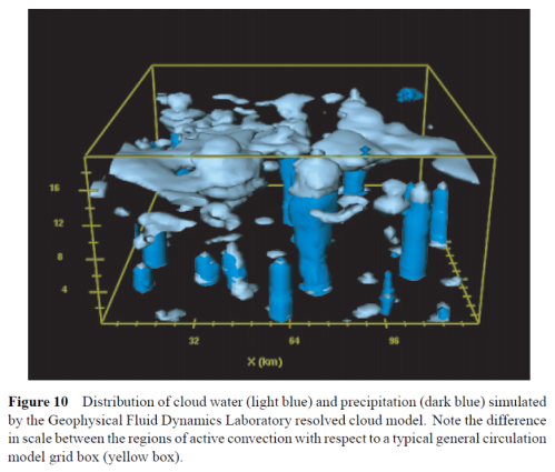
One of the big challenges in climate modeling (there are many) is model resolution and “sub-grid parameterization”. A climate model is created by breaking up the atmosphere (and ocean) into “small” cells of something like 200km x 200km, assigning one value in each cell for parameters like N-S wind, E-W wind and up-down wind – and solving the set of equations (momentum, heat transfer and so on) across the whole earth. However, in one cell like this below you have many small regions of rapidly ascending air (convection) topped by clouds of different thicknesses and different heights and large regions of slowly descending air:
Held and Soden (2000)
The model can’t resolve the actual processes inside the grid. That’s the nature of how finite element analysis works. So, of course, the “parameterization schemes” to figure out how much cloud, rain and humidity results from say a warming earth are problematic and very hard to verify.
Running higher resolution models helps to illuminate the subject. We can’t run these higher resolution models for the whole earth – instead all kinds of smaller scale model experiments are done which allow climate scientists to see which factors affect the results.
Here is the “plain language summary” from Organization of tropical convection in low vertical wind shears:Role of updraft entrainment, Tompkins & Semie 2017:
Thunderstorms dry out the atmosphere since they produce rainfall. However, their efficiency at drying the atmosphere depends on how they are arranged; take a set of thunderstorms and sprinkle them randomly over the tropics and the troposphere will remain quite moist, but take that same number of thunderstorms and place them all close together in a “cluster” and the atmosphere will be much drier.
Previous work has indicated that thunderstorms might start to cluster more as temperatures increase, thus drying the atmosphere and letting more infrared radiation escape to space as aresult – acting as a strong negative feedback on climate, the so-called iris effect.
We investigate the clustering mechanisms using 2km grid resolution simulations, which show that strong turbulent mixing of air between thunderstorms and their surrounding is crucial for organization to occur. However, with grid cells of 2 km this mixing is not modelled explicitly but instead represented by simple model approximations, which are hugely uncertain. We show three commonly used schemes differ by over an order of magnitude. Thus we recommend that further investigation into the climate iris feedback be conducted in a coordinated community model intercomparison effort to allow model uncertainty to be robustly accounted for.
And a little about computation resources and resolution. CRMs are “cloud resolving models”, i.e. higher resolution models over smaller areas:
In summary, cloud-resolving models with grid sizes of the order of 1 km have revealed many of the potential feed-back processes that may lead to, or enhance, convective organization. It should be recalled however, that these studies are often idealized and involve computational compromises, as recently discussed in Mapes [2016]. The computational requirements of RCE experiments that require more than 40 days of integration still largely prohibit horizontal resolutions finer than 1 km. Simulations such as Tompkins [2001c], Bryan et al. [2003], and Khairoutdinov et al. [2009] that use resolutions less than 350 m were restricted to 1 or 2 days. If water vapor entrainment is a factor for either the establishment and/or the amplification of convective organization, it raises the issue that the organization strength in CRMs model using grid sizes of the order of 1 km or larger is likely to be sensitive to the model resolution and simulation framework in terms of the choice of subgrid-scale diffusion and mixing.
In their conclusion on what resolution is needed:
.. and states that convergence is achieved when the most energetic eddies are well resolved, which is not the case at 2 km, and Craig and Dornbrack [2008] also suggest that resolving clouds requires grid sizes that resolve the typical buoyancy scale of a few hundred meters. The present state of the art of LES is represented by Heinze et al. [2016], integrating a model for the whole of Germany with a 100 m grid spacing, for a period of 4 days.
They continue:
The simulations in this paper also highlight the fact that intricacies of the assumptions contained in the parameterization of small- scale physics can strongly impact the possibility of crossing the threshold from unorganized to organized equilibrium states. The expense of such simulations has usually meant that only one model configuration is used concerning assumptions of small-scale processes such as mixing and microphysics, often initialized from a single initial condition. The potential of multiple equilibria and also an hysteresis in the transition between organized and unorganized states [Muller and Held, 2012], points to the requirement for larger integration ensembles employing a range of initial and boundary conditions, and physical parameterization assumptions. The ongoing requirements of large-domain, RCE numerical experiments imply that this challenge can be best met with a community-based, convective organization model intercomparison project (CORGMIP).
Here is Detailed Investigation of the Self-Aggregation of Convection in Cloud-Resolving Simulations, Muller & Held (2012). The second author is Isaac Held, often referenced on this blog who has been writing very interesting papers for about 40 years:
It is well known that convection can organize on a wide range of scales. Important examples of organized convection include squall lines, mesoscale convective systems (Emanuel 1994; Holton 2004), and the Madden– Julian oscillation (Grabowski and Moncrieff 2004). The ubiquity of convective organization above tropical oceans has been pointed out in several observational studies (Houze and Betts 1981; WCRP 1999; Nesbitt et al. 2000)..
..Recent studies using a three-dimensional cloud resolving model show that when the domain is sufficiently large, tropical convection can spontaneously aggregate into one single region, a phenomenon referred to as self-aggregation (Bretherton et al. 2005; Emanuel and Khairoutdinov 2010). The final climate is a spatially organized atmosphere composed of two distinct areas: a moist area with intense convection, and a dry area with strong radiative cooling (Figs. 1b and 2b,d). Whether or not a horizontally homogeneous convecting atmosphere in radiative convective equilibrium self-aggregates seems to depend on the domain size (Bretherton et al. 2005). More generally, the conditions under which this instability of the disorganized radiative convective equilibrium state of tropical convection occurs, as well as the feedback responsible, remain unclear.
We see the difference in self-aggregation of convection between the two domain sizes below:
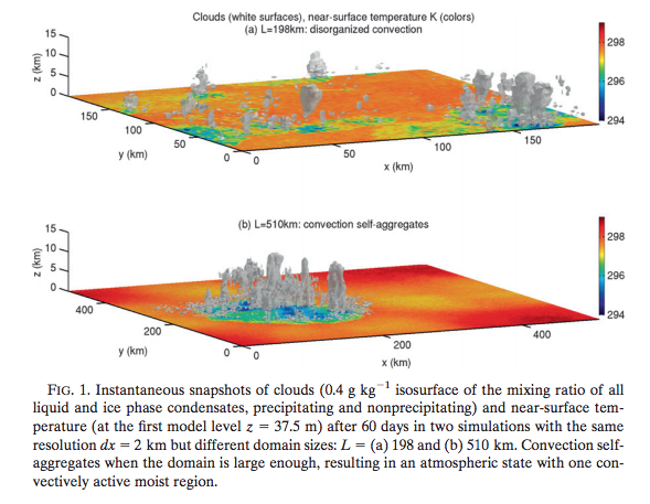
From Muller & Held 2012
Figure 1
The effect on rainfall and OLR (outgoing longwave radiation) is striking, and also note that the mean is affected:
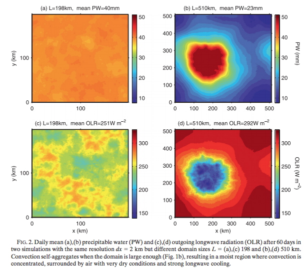
From Muller & Held 2012
Figure 2
Then they look at varying model resolution (dx), domain size (L) and also the initial conditions. The higher resolution models don’t produce the self-aggregation, but the results are also sensitive to domain size and initial conditions. The black crosses denote model runs where the convection stayed disorganized, the red circles where the convection self-aggregated:
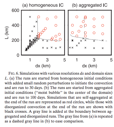
From Muller & Held 2012
Figure 3
In their conclusion:
The relevance of self-aggregation to observed convective organization (mesoscale convective systems, mesoscale convective complexes, etc.) requires further investigation. Based on its sensitivity to resolution (Fig. 6a), it may be tempting to see self-aggregation as a numerical artifact that occurs at coarse resolutions, whereby low-cloud radiative feedback organizes the convection.
Nevertheless, it is not clear that self-aggregation would not occur at fine resolution if the domain size were large enough. Furthermore, the hysteresis (Fig. 6b) increases the importance of the aggregated state, since it expands the parameter span over which the aggregated state exists as a stable climate equilibrium. The existence of the aggregated state appears to be less sensitive to resolution than the self-aggregation process. It is also possible that our results are sensitive to the value of the sea surface temperature; indeed, Emanuel and Khairoutdinov (2010) find that warmer sea surface temperatures tend to favor the spontaneous self-aggregation of convection.
Current convective parameterizations used in global climate models typically do not account for convective organization.
More two-dimensional and three dimensional simulations at high resolution are desirable to better understand self-aggregation, and convective organization in general, and its dependence on the subgrid-scale closure, boundary layer, ocean surface, and radiative scheme used. The ultimate goal is to help guide and improve current convective parameterizations.
From the results in their paper we might think that self-aggregation of convection was a model artifact that disappears with higher resolution models (they are careful not to really conclude this). Tompkins & Semie 2017 suggested that Muller & Held’s results may be just a dependence on their sub-grid parameterization scheme (see note 1).
From Hohenegger & Stevens 2016, how convection self-aggregates over time in their model:
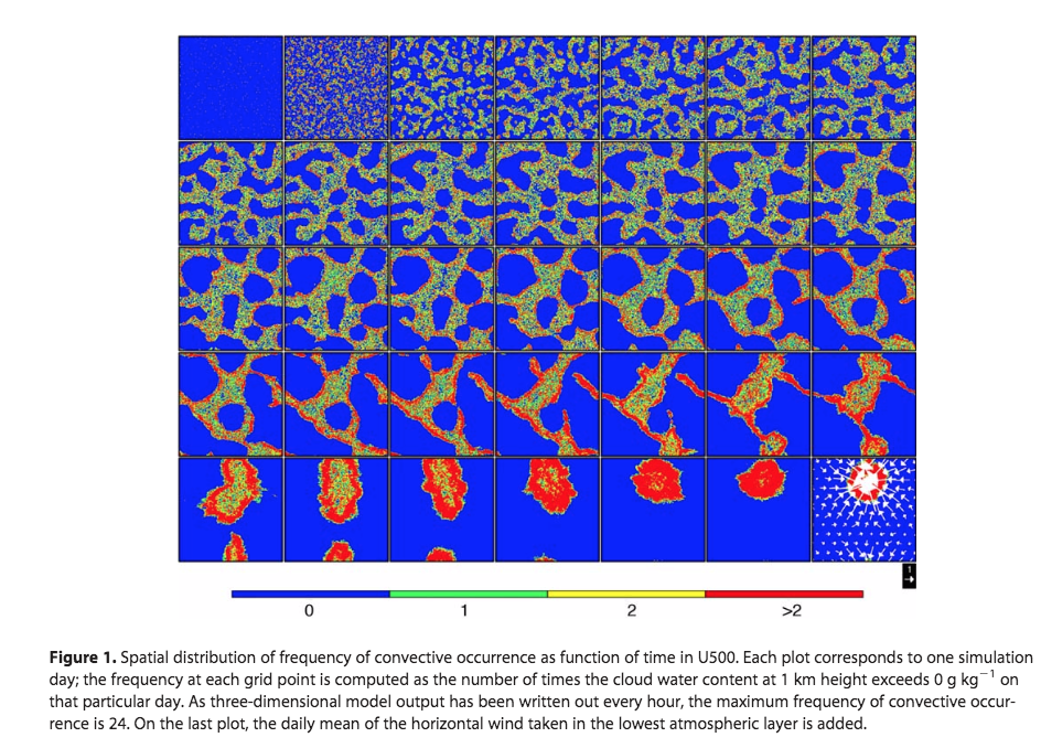
From Hohenegger & Stevens 2016
Figure 4 – Click to enlarge
From a review paper on the same topic by Wing et al 2017:
The novelty of self-aggregation is reflected by the many remaining unanswered questions about its character, causes and effects. It is clear that interactions between longwave radiation and water vapor and/or clouds are critical: non-rotating aggregation does not occur when they are omitted. Beyond this, the field is in play, with the relative roles of surface fluxes, rain evaporation, cloud versus water vapor interactions with radiation, wind shear, convective sensitivity to free atmosphere water vapor, and the effects of an interactive surface yet to be firmly characterized and understood.
The sensitivity of simulated aggregation not only to model physics but to the size and shape of the numerical domain and resolution remains a source of concern about whether we have even robustly characterized and simulated the phenomenon. While aggregation has been observed in models (e.g., global models) in which moist convection is parameterized, it is not yet clear whether such models simulate aggregation with any real fidelity. The ability to simulate self-aggregation using models with parameterized convection and clouds will no doubt become an important test of the quality of such schemes.
Understanding self-aggregation may hold the key to solving a number of obstinate problems in meteorology and climate. There is, for example, growing optimism that understanding the interplay among radiation, surface fluxes, clouds, and water vapor may lead to robust accounts of the Madden Julian oscillation and tropical cyclogenesis, two long-standing problems in atmospheric science.
Indeed, the difficulty of modeling these phenomena may be owing in part to the challenges of simulating them using representations of clouds and convection that were not designed or tested with self-aggregation in mind.
Perhaps most exciting is the prospect that understanding self-aggregation may lead to an improved understanding of climate. The strong hysteresis observed in many simulations of aggregation—once a cluster is formed it tends to be robust to changing environmental conditions—points to the possibility of intransitive or almost intransitive behavior of tropical climate.
The strong drying that accompanies aggregation, by cooling the system, may act as a kind of thermostat, if indeed the existence or degree of aggregation depends on temperature. Whether or how well this regulation is simulated in current climate models depends on how well such models can simulate aggregation, given the imperfections of their convection and cloud parameterizations.
Clearly, there is much exciting work to be done on aggregation of moist convection.
[Emphasis added]
Conclusion
Climate science asks difficult questions that are currently unanswerable. This goes against two myths that circulate media and many blogs: on the one hand the myth that the important points are all worked out; and on the other hand the myth that climate science is a political movement creating alarm, with each paper reaching more serious and certain conclusions than the paper before. Reading lots of papers I find a real science. What is reported in the media is unrelated to the state of the field.
At the heart of modeling climate is the need to model turbulent fluid flows (air and water) and this can’t be done. Well, it can be done, but using schemes that leave open the possibility or probability that further work will reveal them to be inadequate in a serious way. Running higher resolution models helps to answer some questions, but more often reveals yet new questions. If you have a mathematical background this is probably easy to grasp. If you don’t it might not make a whole lot of sense, but hopefully you can see from the papers that very recent papers are not yet able to resolve some challenging questions.
At some stage sufficiently high resolution models will be validated and possibly allow development of more realistic parameterization schemes for GCMs. For example, here is Large-eddy simulations over Germany using ICON: a comprehensive evaluation, Reike Heinze et al 2016, evaluating their model with 150m grid resolution – 3.3bn grid points on a sub-1 second time step over 4 days over Germany:
These results consistently show that the high-resolution model significantly improves the representation of small- to mesoscale variability. This generates confidence in the ability to simulate moist processes with fidelity. When using the model output to assess turbulent and moist processes and to evaluate and develop climate model parametrizations, it seems relevant to make use of the highest resolution, since the coarser-resolved model variants fail to reproduce aspects of the variability.
Related Articles
Ensemble Forecasting – why running a lot of models gets better results than one “best” model
Latent heat and Parameterization – example of one parameterization and its problems
Turbulence, Closure and Parameterization – explaining how the insoluble problem of turbulence gets handled in models
Part Four – Tuning & the Magic Behind the Scenes – how some important model choices get made
Part Five – More on Tuning & the Magic Behind the Scenes – parameterization choices, aerosol properties and the impact on temperature hindcasting, plus a high resolution model study
Part Six – Tuning and Seasonal Contrasts – model targets and model skill, plus reviewing seasonal temperature trends in observations and models
References
Missing iris efect as a possible cause of muted hydrological change and high climate sensitivity in models, Thorsten Mauritsen and Bjorn Stevens, Nature Geoscience (2015) – free paper
Organization of tropical convection in low vertical wind shears:Role of updraft entrainment, Adrian M Tompkins & Addisu G Semie, Journal of Advances in Modeling Earth Systems (2017) – free paper
Detailed Investigation of the Self-Aggregation of Convection in Cloud-Resolving Simulations, Caroline Muller & Isaac Held, Journal of the Atmospheric Sciences (2012) – free paper
Coupled radiative convective equilibrium simulations with explicit and parameterized convection, Cathy Hohenegger & Bjorn Stevens, Journal of Advances in Modeling Earth Systems (2016) – free paper
Convective Self-Aggregation in Numerical Simulations: A Review, Allison A Wing, Kerry Emanuel, Christopher E Holloway & Caroline Muller, Surv Geophys (2017) – free paper
Large-eddy simulations over Germany using ICON: a comprehensive evaluation, Reike Heinze et al, Quarterly Journal of the Royal Meteorological Society (2016)
Other papers worth reading:
Featured Article Self-aggregation of convection in long channel geometry, Allison A Wing & Timothy W Cronin, Quarterly Journal of the Royal Meteorological Society (2016) – paywall paper
Notes
Note 1: The equations for turbulent fluid flow are insoluble due to the computing resources required. Energy gets dissipated at the scales where viscosity comes into play. In air this is a few mm. So even much higher resolution models like the cloud resolving models (CRMs) with scales of 1km or even smaller still need some kind of parameterizations to work. For more on this see Turbulence, Closure and Parameterization.


And an interesting comment in the conclusion of a very interesting paper – Radiative convective equilibrium as a framework for studying the interaction between convection and its large-scale environment, Levi G Silvers, Bjorn Stevens, Thorsten Mauritsen & Marco Giorgetta, Journal of Advances in Modeling Earth Systems (2016):
This echoes my comment in Climate Sensitivity – Stevens et al 2016 about the problems of non-linear systems.
This paper has two co-authors we have already met and is freely available.
Wait… So maybe that fool Lindzen was right all along? Shocking.
Seems to me that convection should naturally organize itself to maximize heat flow from the surface to space. Convection forms as a response to a surface temperature which is higher than the potential temperature aloft, and disappears when that difference is gone.
Enh, the problem wasn’t that Lindzen’s Iris ideas were fundamentally untenable — they weren’t — but that he pushed them much harder than the evidence warranted, even when evidence was pointing the other way. It was like he had an emotional attachment to his ideas that went further than the evidence. Scientists have a duty to be duly skeptical of their own ideas; “the easiest person to fool is yourself”.
And Lindzen was also caught being deceptive when communicating with the public about climate change…
http://www.realclimate.org/index.php/archives/2012/03/misrepresentation-from-lindzen/
https://skepticalscience.com/skepticquotes.php?s=6
Anyways, back on the Iris ideas.. this is pretty neat stuff. It will be interesting to see how it resolves.
In the pantheon of “fool yourself” scientists, Lindzen seems not even a good example, and especially not when compared to several well known climate scientists.
Windchaser,
I refer you to the case of Wegener and continental drift. The powers that be in the scientific community didn’t like Wegener and, admittedly, his mechanism was cr@p. But the physical evidence that continents had been joined was overwhelming to anyone with half a brain. Yet the dogma of fixed continents persisted for decades.
Thanks SOD. This is not surprising since convection is a classical ill-posed problem. The shear layers form a cascade of eddies that are chaotic. I wonder how more efficient convection would change the vertical temperature profile in the topics, but know vastly too little to hazard a guess.
With respect, I feel like you’re using “climate” more or less interchangeably with atmospheric physics/meteorology in some places:
“At the heart of modeling climate is the need to model turbulent fluid flows (air and water) and this can’t be done.”
for example.
Is this really true of “climate”? Or more to the point, is it really meaningful? I’d argue that it depends on the context of the question, and for many “climate” questions, topics like this one are basically irrelevant. From a paleo perspective, for example, or an extra-terrestrial/exo-planetary perspective, the questions being asked are qualitative enough that I’m not sure the presence or absence of an iris like effect matter much at all.
Do you think perhaps there’s a forest for the trees problem with making sweeping claims like the one I quoted?
Peter,
Yes, it is true of climate. Non-linear processes don’t just sort themselves out.
In a warming world what will happen to clouds? Will there be more or less? –
– Clouds cool the climate, by about 20W/m2 (the net result of two larger effects of a warming and a cooling).
– How much water vapor will there be in the mid-troposphere? Water vapor is a very powerful greenhouse gas.
If you read the papers I cited you find that the reason climate scientists work on these problems is because it matters for climate.
Right now climate models – which by no means are sampling all the uncertainties in our understanding of climate processes – suggest anything from an increase of 1.5’C to 4.5’C from doubling CO2. Do you know the reason why current models have such a huge range?
SOD: Apparently one can observe large differences in convection even even with traditional grid cell size.
Zhao, M. et al. Uncertainty in Model Climate Sensitivity Traced to Representations of Cumulus Precipitation Microphysics. Journal of Climate 29, 543–560 (2016). http://journals.ametsoc.org/doi/pdf/10.1175/JCLI-D-15-0191.1
Uncertainty in equilibrium climate sensitivity impedes accurate climate projections. While the intermodel spread is known to arise primarily from differences in cloud feedback, the exact processes responsible for the spread remain unclear. To help identify some key sources of uncertainty, the authors use a developmental version of the next-generation Geophysical Fluid Dynamics Laboratory global climate model (GCM) to construct a tightly controlled set of GCMs where only the formulation of convective precipitation is changed. The different models provide simulation of present-day climatology of comparable quality compared to the model ensemble from phase 5 of CMIP (CMIP5). The authors demonstrate that model estimates of climate sensitivity can be strongly affected by the manner through which cumulus cloud condensate is converted into precipitation in a model’s convection parameterization, processes that are only crudely accounted for in GCMs. In particular, two commonly used methods for converting cumulus condensate into precipitation can lead to drastically different climate sensitivity, as estimated here with an atmosphere–land model by increasing sea surface temperatures uniformly and examining the response in the top-of-atmosphere energy balance. The effect can be quantified through a bulk convective detrainment efficiency, which measures the ability of cumulus convection to generate condensate per unit precipitation. The model differences, dominated by shortwave feedbacks, come from broad regimes ranging from large-scale ascent to subsidence regions. Given current uncertainties in representing convective precipitation microphysics and the current inability to find a clear observational constraint that favors one version of the authors’ model over the others, the implications of this ability to engineer climate sensitivity need to be considered when estimating the uncertainty in climate projections.
“drastically different climate sensitivity” = ECS 3.0 vs. 1.8
I am aware of the issues discussed in your post. I think they’re interesting. I don’t think they mean we can’t model climate because we can’t model turbulent flows. I proposed that might be missing the forest for the trees.
A zero dimensional energy balance equation is a climate model, as you are yourself aware. So I contend that you’re talking about something more specific than “climate” when you make the claim “at the heart of modeling climate is the need to model turbulent fluid flows (air and water) and this can’t be done.”
>In a warming world what will happen to clouds? Will there be more or less?
They may negate a little warming, they might substantially increase the warming. There is uncertainty. Is it meaningful? Not in the contexts in which many work. Most likely clouds will increase warming, but only moderately. There is virtually no credible evidence that they will act as even a moderately negative feedback. To some people, the question that dominates their lives is what the precise outcome to this question will be. To others, it’s counting angels on the head of a pin. Does not the significance of this question depend on one’s context? If I am a policymaker, my uncertainty is not dominated by the magnitude of the cloud feedback or the value of ECS, it’s dominated by our emissions trajectory. If I am a paleoclimate researcher, it’s dominated by less well-constrained boundary conditions. If I am an exoplanet researcher, I may not even have clouds to worry about. But all of these other foci are still concerned with, still modeling, climate.
If you believe that we cannot model the climate because we cannot explicitly model certain cloud-related processes, that’s of course your prerogative. I was hoping to interrogate that premise in a way that would allow for some sort of productive dialog. But if instead you have an immutable opinion on this and wish to redirect with climate 101 stuff, this isn’t the place for me.
Thanks for reading. Fingers crossed.
Peter,
“All models are wrong but some are useful” is a useful way to think about climate models.
We can do a basic 1d energy calculation with a doubling of CO2 and see that with absolute humidity fixed the surface temperature needs to rise by about 1.2’C to bring the climate back into balance. Or with relative humidity fixed the surface temperature needs to rise by about 2.5’C (different people got different numbers back in the past). This is a very useful model. Then instead of calculating on one “US standard atmosphere” we can check at multiple points across the globe, area average, and get – well, basically similar values – another useful model.
So in that sense you are right, modeling turbulent fluid flows is not at the heart of modeling climate.
I’m interested in how reliable their temperature projections are (along with rainfall and others items) and reducing the bounds of uncertainty. So are many climate scientists. To do this requires modeling turbulent fluid flows.
I like your style after our long discussion – “immutable opinion“. I can see my obstinate approach brought into focus now.
Instead of me pinning some faintly damning label on you based on my interpretation of your thinking based on your two comments today let’s try an alternative.
Do you think the difference between 1.5K warming and 4.5K is about being precise?
The most recent IPCC report (AR5) said for RCP6 (which is close enough to doubling CO2) –
“Under the assumptions of the concentration-driven RCPs, global mean surface temperatures for 2081–2100, relative to 1986–2005 will likely be in the 5 to 95% range of the CMIP5 models: 1.4°C to 3.1°C – RCP6″
This is a narrower range than some climate scientists discuss.
For example, in “Broad range of 2050 warming from an observationally constrained large climate model ensemble”, Daniel J. Rowlands et al, Nature (2012) they try to sample the uncertainty of climate models a little more and of course find a wider range. Likewise they have the same approach in: “Uncertainty in predictions of the climate response to rising levels of greenhouse gases”, DA Stainforth et al, Nature (2005).
Climate models also struggle with rainfall – this is most likely a consequence of not resolving the climate sufficiently, along with uncertainty on many microphysical processes. Rainfall projections for important areas like the Sahel in the late 21st century vary from “less rainfall” to “more rainfall” to “extreme rainfall”. Monsoon regions likewise.
We have huge uncertainty. Narrowing the range has immense value. If the global average temperature change from 2xCO2 is worked out to be an increase of 1.5’C or 1’C rather than 3’C or 4’C this will be immensely valuable data. Likewise, if we can actually determine some range for smaller areas where people live (e.g. California, NW Europe) along with rainfall changes this will have huge benefits.
I can’t think that precise is the term to use. Right now RCP6 tells a given region the late 21st century will be “warmer” and “maybe wetter or drier” with higher sea level.
Over to you.
Peter, Perhaps a more correct statement is that GCM’s can’t model climate accurately without some model of turbulence that goes beyond traditional eddy viscosity models that are really mostly based on boundary layer theory and test data. Simple models can in some cases of course be tuned to fit the data pretty well. That’s not a contradiction.
With that thought above from dpy6629 in my mind, having just clicked open the wrong Sandrine Bony paper to read – Marine boundary layer clouds at the heart of tropical cloud feedback uncertainties in climate models, Sandrine Bony & Jean-Louis Dufresne, GRL (2005) – but read it anyway:
Emphasis added.
This (highlighted) problem is a key element of climate models, and models from many other fields with unknown parameters and especially sub-grid parameterizations.
SOD and Peter: When you mention marine boundary layer clouds, it is worth remembering that the relative humidity of the boundary layer is projected to increase. This happens because overturning of the atmosphere slows and precipitation can’t increase at 7%/K. The increase in relative humidity appears small (80% to 81%), but is much larger when expressed in terms of “undersaturation” (20% to 19%). This is a 5% change in undersaturation, which produces a 5% reduction in evaporation and brings marine boundary layer 5% closer to condensation.
SOD wrote: “Or with relative humidity fixed the surface temperature needs to rise by about 2.5’C.”
However, the constant relative humidity assumption model is physically improbable, because it transfers far more latent heat (5.6 W/m2/K) into the atmosphere after warming than can possibly be consistent with an ECS of 2.5 degC – a 1.5 W/m2/K increase in OLR and reflected SWR at the TOA.
We can ignore convection and make whatever assumptions we want about constant relative or absolute humidity and clouds, but climate is all about radiative cooling to space. CO2 is only a small part of that story. Only 10% of TOA OLR originates from the surface. It would be interesting to know what fraction is emitted from clouds, what fraction by water vapor, and what fraction is emitted by CO2. Relative humidity drops with altitude because of convection and clouds are created by convection. And we should include reflection of SWR back to space as part of radiative cooling. 2/3rds of the planet is covered by clouds that reflect an average of 125 W/m2 back to space while the surface reflects 50 W/m2 (according to CERES).
My first comment posted immediately. The second is not. Don’t know if that means it’s in an approval queue or if it did not go through…
I don’t see it. I also checked the sp&m queue but there’s nothing there from you.
Reply from Peter Jacobs (received via email):
Okay, the quick summary version…
You fairly dinged me on tone. I admit I was a little snarky because your comments seemed a little condescending. I am not a cloud specialist, but I am currently doing a CESM run on Cheyenne with an altered ice and liquid water path radiation scheme so I am not exactly unfamiliar with the basics of clouds and climate change.
Do you think that ECS is plausibly as low as 1C? That’s shocking.
Do I think ECS is bounded between 1.5-4.5C? No. Climate models are only one line of evidence for ECS. Paleoclimate and observational constraints also exist. Moreover, the models that best reproduce observed features of the system, be they processes important to feedbacks or just broad scale trends like temperature or Arctic sea ice, generally don’t have ECS values lower than 2.
Even if ECS was on the lower end of plausible values, that would mean little from a policy perspective. A decade’s worth of emissions, basically (Rogelj 2014). That changes nothing about the big questions we face (do we need to cut emissions to stay below a given target, do we need to start now).
I am not saying we have sensitivity perfectly solved. I am saying that a TCR of 1.8C give or take an ECS of 3C give or take is consistent with many lines of evidence.
If you want to talk about state-level projections a few decades out, uncertainty is greater but then again that strikes me much less as a “climate” question rather than a pretty narrow subset of climate that you just happen to be interested in.
What else did I miss?
Oh, so perhaps I was reading into your comments things that you did not intend. If so, my apologies. So rather than assume, I will ask.
Do you agree that the cloud feedback is most likely positive, very likely modest or small, and almost certainly not a large negative feedback? Why do you think people who have spent much of their careers studying cloud-climate impacts like Tony Del Genio and Andy Dessler think the question of clouds is not entirely solved but is pretty well constrained? Do you agree that the tropospheric water vapor feedback is positive? Do you agree that there are plenty of aspects of climate in which resolving turbulent flows either doesn’t come into play or is not the important source of uncertainty?
What else? Oh. The Royal Society recently published an update to the state of knowledge since the AR5. It discussed our understanding of sensitivity and stated that values of ECS below 2C were found to be less plausible.
There was more but it’s late and I can’t remember what else. If it comes to me I will post a follow up.
Peter Jacobs,
Sorry, I didn’t mean to sound or be condescending. Lots of unknown new people arrive and ask questions, make comments, make claims. Some know nothing of even thermodynamics basics, some know nothing of climate modeling. Many of these have grand ideas unsupported by reality. Some arrive with lots of knowledge and insights, we even once had a visit from the great Prof. Pierrehumbert (it was more like his book promotion tour and I did buy it). Anyway, hard to pitch an answer to a short question from an unknown person.
More on your other points later.
No, seems very unlikely. It was just a for instance, probably primed by Bjorn Stevens paper referenced in the last article on this site. Of course, he is likewise giving lines of evidence for ruling out various values. Think of it as a throwaway line.
Seems highly likely. I can’t imagine that it could be negative. The simplest most sensible approach in the absence of recent detailed data is what Manabe and Wetherald did (1967) and held relative humidity constant. But of course that is just a finger in the air approach.
How positive is tricky because upper tropospheric water vapor is really the key (for affecting the radiation balance), the concentration is minute compared with boundary layer concentration and the dependencies are mostly in the convection schemes and.. turbulent flows.
On the first item, I don’t know.
On the second item I don’t know.
You probably have the second one as a rhetorical question. This blog has the principle of scientific enquiry and evidence rather than “top blokes” idea.
Of course, the first place I go to find out about a difficult subject is the people who have been studying it for a long time because they will know minimum 100x more about it than me. And if I can’t understand their reasoning I start by assuming I am missing something – for the exact same reason. But in the end, it’s about the strength of evidence. (See note below for example).
You might now be assuming that I think clouds are a negative feedback (I’m not assuming you are assuming but just in case). No. I don’t know. I always want to read more so suggest some papers. I have read a bunch of Dessler papers:

Fundamentally our understanding of the response of clouds is a problem of processes not resolved by climate models and our observations are very limited. I’m hoping AIRS and CERES will give us the big idea that we need to simplify the problem but that might not happen (maybe it already has?).
Anyway, suggestions on cloud papers appreciated.
—
(Unrelated/semi-related) Note: I read the entire chapter (ch 10) on attribution in AR5, read countless papers referenced and followed all of their references going back to Hasselmann 1993 and my conclusion (see Natural Variability and Chaos – Three – Attribution & Fingerprints) was it was made up stats. They are giants in the field and I’m just a statistical novice. But so what, in the end.
Funnily enough the authors of chapter 11 of AR5 also agreed with me. They put their finger in the air and downgraded the “almost certain” to “quite likely” with zero analysis of whether is was in fact “quite likely”, “as likely as likely not” “quite unlikely” and so on.
I’m sure the authors of chapter 10 believed their 95% and they have countless papers to their eminent names.
Peter,
When you said “Rogelj 2014” did you mean “Air-pollution emission ranges consistent with the representative concentration pathways”?
Can you provide some references?
Plenty? On balance I’ll say no.
Other important sources of uncertainty come from:
– the carbon cycle (relating emissions to CO2 in the atmosphere, even more difficult for CH4)
– vegetation feedbacks
Every paper on climate sensitivity not related to the carbon cycle or vegatation that I can think of has been an unspoken result of, or a noted result of, turbulent flows. That is, clouds and water vapor feedbacks.
I’m interested in the counter-argument – that is what this blog is for.
Reply from Peter (not able to post due to some WordPress issue):
Thanks for posting my half-remembered comment. Some follow up.
I am no Ray Pierrehumbert, and I am not trying to make appeals to authority on my own behalf. I am just a PhD student who does some climate modeling and some stuff on modern instrumental biases but mainly is interested in paleoclimate and marine ecosystem impacts.
My references to Tony Del Genio and Andy Dessler were likewise not appeals to authority, they were genuine questions. I think asking those questions helps cut through a lot of confusion. Putting oneself in the frame of reference of other people tends to ameliorate some cognitive biases which we’re all susceptible to. There are of course instances in which a motivated amateur comes to a very different conclusion than domain experts and dramatically changes a field, but these are a vanishingly small handful of exceptions rather than the rule. Let us consider: what these domain experts may know that we don’t know?
I am also not an optimal fingerprinting/attribution specialist, but I have done a little research in that area. I don’t think I quite agree with the link you provided, but that might be off-topic for this particular thread.
It sounds like you think that there is some non-trivial possibility for a large negative cloud feedback. I would contend that there is not really any “room” for such a large and unaccounted for negative feedback given what we know from observations, paleoclimate, theory, etc. A lot of other things would have to be wrong that we have no reason to believe are wrong (and have good reason to believe are right, or at least decently bounded). I’m happy to discuss this at further length as it is more or less the subject of this post. However my initial comment/question was how necessary modeling turbulent flows was to the subject of climate. I was contending that it may be very necessary in some context, but not necessarily for the broad topic itself.
In many instances such as paleoclimate reconstructions, modeling climate impacts, for many kinds of observational climate work, etc., things don’t hinge in any meaningful way on the ability to model turbulent flows.
> did you mean “Air-pollution emission ranges consistent with the representative concentration pathways”
No. I meant doi:10.1088/1748-9326/9/3/031003 (trying to avoid the sp_m filter).
More later.
Peter,
Of course, this a good point.
But the best approach is – cite a paper, or multiple papers, or a line of evidence, that is what we are looking for.
– Why do x and y believe something? I have no idea.
– What do you make of the evidence presented in this paper? That’s a good question and now I have something to get my teeth into.
Peter wrote to SOD: “It sounds like you think that there is some non-trivial possibility for a large negative cloud feedback. I would contend that there is not really any “room” for such a large and unaccounted for negative feedback given what we know from observations, paleoclimate, theory, etc.
It would be interesting to hear more about the evidence supports this position.
Paleoclimate: On a long time scale, our planet oscillates from interglacial to glacial periods without clear evidence of a GLOBAL change in forcing that can be amplified by feedbacks. SOD has written a long series of posts on this subject showing that there is no one theory that explains this phenomena. IMO, any deductions might be made about climate sensitivity in general and specifically about cloud feedback shouldn’t be applied to today’s radically different interglacial period (5 K warmer, more rainfall, less dust, 120 m higher ocean, different surface albedo) and certainly shouldn’t be extended to an 8-10+K warmer future. I would agree that our climate appears unstable towards cooling, but I can’t formulate this in terms of a forcing amplified by a climate feedback parameter that is near zero because of cloud feedback.
Models vs Observations: Every year the planet warms 3.5 K during summer in the NH because of the lower heat capacity of this hemisphere (but this seasonal signal is normally eliminated by working with temperature and flux anomalies). Every year this produces massive changes in TOA OLR and reflected SWR (Ie feedbacks) from both clear and cloudy skies that reliable climate models should be able to reproduce. However, models disagree substantially WITH EACH OTHER and with OBSERVATIONS about cloud LWR and SWR feedback (and surface albedo feedback).
http://www.pnas.org/content/110/19/7568.full
The gain factors of longwave feedback that operates on the annual variation of the global mean surface temperature. (A) All sky. (B) Clear sky. (C) Cloud radiative forcing. Blank bars on the left indicate the gain factors obtained from satellite observation (ERBE, CERES SRBAVG, and CERES EBAF) with the SE bar. Black bars indicate the gain factors obtained from the models identified by acronyms at the bottom of the figure (Methods, Data from Models). The vertical line near the middle of each frame separates the CMIP3 models on the left from the CMIP5 models on the right.
The gain factors of solar feedback that operate on the annual variation of the global mean surface temperature. (A) All sky. (B) Clear sky. (C) Cloud radiative forcing. See Fig. 3 legend for further explanation.
I tried again, same result. If it doesn’t show up again in the morning I will try a shorter comment. I saved the second try in a text file…
Does it say “Comment in moderation” or nothing and it disappeared?
Nothing. The page reloaded after I clicked ‘post comment’ the same as it does when the first comment went through but nothing is added.
And if you like you can email it to scienceofdoom- you know what goes here -gmail.com and I’ll post it.
WordPress shows me 3 queues: approved (automatic), moderation (catches key words, particular commenters – but emails me to tell me there is a comment in moderation), sp&m (it decides what goes in here without asking or telling me).
None of these have your comment. Maybe WordPress is having a bad day.
I have contacted a WordPress “happiness engineer” for assistance. They have been very helpful in the past and restored my happiness.
An interesting paper for readers new to ensembles of model results: Ensemble modeling, uncertainty and robust predictions, Wendy S. Parker, WIREs Clim Change 2013.
There are lots of papers saying the same thing – like in many fields – without much new to add. This paper fits squarely into that category but at least explains the topic reasonably well.
slides of some sort for unpublished Dessler, Mauritzen, and Stevens: A revision of the Earth’s energy balance framework
So if I read that right, ECS is between 1.5 and 3.5K for doubling CO2. That’s pretty close to Steven Mosher’s original lukewarmer position of 1.5 to 3K.
JCH,
Thanks, very interesting – as always when you get someone’s slides you miss all the useful points. I emailed the main contact for that conference to ask if there was more from Dessler’s talk, and for the other presentations.
CFMIP 2017.
The Meeting on Clouds, Precipitation, Circulation, and Climate Sensitivity will be held 25-28 September 2017 at Itoh Hall, Hongo Campus, University of Tokyo, Tokyo, Japan.
This CFMIP international meeting will focus on the theme of the WCRP Grand Challenge on Clouds, Circulation and Climate Sensitivity, in addition to addressing other ongoing CFMIP activities.
The enforcers must really be after Stevens because boy that guy is in on a lot of papers!
Scroll down to the very last graphic. It says 11 of 11 models, with a red star at around 2.8.
Is anyone able to enlighten me on this slide (slide #14):
It’s a long time since I went on a journey through climate sensitivity..
If the models and observations have the same values, why is ECS different for the two cases. It’s probably ECS 101 and I missed it..
I agree that ECS should be the same in the two cases. Also, if there is a specific value of lambda, there should be a specific value of ECS (or only a very small range).
It looks like he might be saying that the forcing, TOA imbalance, and change in surface T are the same in models and the data (but they aren’t). And then saying that it is puzzling why the observations (using simple energy balance) don’t give the same sensitivity as the models (not using simple energy balance)? But I was never good at reading tea leaves.
I have no idea, but OBS yield a single value and MODELS yield a range?
I think it is the problem of reading slides when no one is talking.
Basically the slide is saying NOT that the values are the same, just that the equation is the same.
I think. It’s the kind of stuff people do on slides – makes no sense when you can’t hear the presenter, perfect sense if you are listening.
Otherwise, the above is impossible.
Is the red star, last graphic, the central estimate?
The red star does appear to be some kind of central estimate… but without the commenary that goes with the pictures, it is hard to say for sure.
I do wonder when models projecting ECS over 4C are going to be either ignored or revised.
SOD asked about slide #14: lambda (the climate sensitivity parameter) is the increase in net flux of heat lost to space (both TOA OLR and reflected SWR) as the surface warms 1 degK. It should have units of W/m2/K (assuming I know what I am talking about, of course). If you assume 3.7 W/m2 for the radiative forcing from 1 doubling of CO2, -1.3 W/m2/K would be an ECS of 2.8 K/doubling and -2 W/m2/K would be 1.85 K/doubling (near what energy balance models predict). 3.7 W/m2/doubling comes from high resolution RTE calculations on typical atmospheric profiles. Each AOGCM produces it own atmospheric profile and a different value for the radiative forcing from 2XCO2 that is extrapolated from abrupt 4XCO2 experiments. (See the fifth slide showing dF)
dR is the radiative imbalance at the TOA (and is approximated by the rate of ocean heat uptake as measure by ARGO). At equilibrium, dR goes to zero (by definition) and dTs = dF/lambda. However, modelers now realize lambda isn’t constant – plots of dR vs dTs are not linear in abrupt 4XCO2 experiments, something Dessler didn’t bother to show. I guessing now, but I think “obs” refers to the historic record of warming (Lewis and Curry) AND model runs that emulate that period, which are consistent with ECS less than or equal to 2 K. The “models” data comes from abrupt 4XCO2 experiments where lambda has shrunk with warming.
With energy balance models, climate sensitivity at any time can be calculated from the transient warming (dTs) in response to the current change in forcing (dF), ocean heat uptake which is also approximately the TOA radiative imbalance.
lambda = (dR – dF)/dTs = (dQ – dF)/dTs
However, this gives us climate sensitivity in units of W/m2/K, the increase in net radiative cooling to space in response to surface warming. To convert this to the usual measure of climate sensitivity (K/doubling), we need to know the forcing from doubled CO2 (F_2x). (The signs come out right if you remember that by convention F_2x, dF and dQ (dR) are all negative.)
ECS = F_2x/lambda = F_2x * dTs/(dF-dQ)
Mike M wrote: “It looks like he might be saying that the forcing, TOA imbalance, and change in surface T are the same in models and the data (but they aren’t). And then saying that it is puzzling why the observations (using simple energy balance) don’t give the same sensitivity as the models (not using simple energy balance)?”
I think CMIP6 modelers are working under some constraints that didn’t apply to CMIP3 and 5. It is possible to that all models may be required to use the same (or at least a plausible) radiative forcing from aerosols when hindcasting historic warming – eliminating or minimizing this controversial fudge factor. The current ocean heat uptake / TOA radiative imbalance has been fairly well established by ARGO, eliminating another mechanism for high ECS models to reduce hindcast warming by sending heat into the deep ocean. So their TCR’s and ECS’s from hindcast data may be constrained to agree with energy balance models. Thus everyone would be working with roughly the same dF and dR (dQ) and wanting their model to predict the historic dTs.
In essence, Lewis and Curry (and Otto et al) have won the debate about the past. However, if feedbacks are not linear and lambda changes with warming (from -2 W/m2/K in the 20th century to -1.3 W/m2/K at the end of abrupt 4XCO2 experiments), models can still produce scary ECS’s.
Frank wrote: “It is possible to that all models may be required to use the same (or at least a plausible) radiative forcing from aerosols when hindcasting historic warming – eliminating or minimizing this controversial fudge factor. The current ocean heat uptake / TOA radiative imbalance has been fairly well established by ARGO, eliminating another mechanism for high ECS models to reduce hindcast warming by sending heat into the deep ocean. So their TCR’s and ECS’s from hindcast data may be constrained to agree with energy balance models. Thus everyone would be working with roughly the same dF and dR (dQ) and wanting their model to predict the historic dTs.”
That would be good news indeed and would be a fine example of climate science acting like a normal science.
SOD: Unless I’m crazy, the slides in Dessler’s talk have changed between yesterday and today. This table is no longer present. Blog policy prevents me from speculating about motives.
Click to access 1-5_Dessler.pdf
Just blog policy preventing you? Not rationality?
You’re linking to a different slideshow pdf than the one with that slide 14 graphic, that’s why it’s different. Neither pdf has been altered in months. I guess blog policy prevents me from speculating why you immediately jumped at an attempt to impugn climate scientists?
Paulski: I clicked the link provided by SOD yesterday. Wanting to point out elsewhere that even Dessler was limiting ECS to a max of 3.5 K (on some slides), I came back to the same link today to find a different set of slides. In my disappointment, I made an unnecessarily snarky remark for which I apologize. I really don’t know what happened, except that the table SOD posted is no longer visible.
SOD wrote: “Masa replied quickly.
It looks like slides (but no talk) are HERE”.
Frank – I provided the link you were looking at: first post on this thread. Still links to the same set of slides.
Thanks JCH. The presentation you linked and the Dessler talk at the conference SOD linked have some things in common, but the latter is four months later.
What’s sad is that I look at this slide and I can’t remember the point I was making, either. Just joking. The question I’m posing here is that if you take observations of forcing, surface temperature, top of atmosphere flux and infer climate sensitivity you get very low values ( 2°C. https://youtu.be/mdoln7hGZYk
However, in talking with colleagues everyone else hated that approach. It was just too qualitative. So now we have a much more qualitative way to do the estimate and come up with a range of 2.4°C to 4.5°C. Here’re some updated slides that show this new approach (note that the numbers are a little different b/c of an issue with the 2xCO2 forcing). http://www.miroc-gcm.jp/cfmip2017/CFMIP_PDF/Day01/1-5_Dessler.pdf
something happened to my response. I think the system doesn’t like less than or greater than signs. Here is is again.
What’s sad is that I look at this slide and I can’t remember the point I was making, either. Just joking. The question I’m posing here is that if you take observations of forcing, surface temperature, top of atmosphere flux and infer climate sensitivity you get very low values (less than 2°C). Climate models using the same forcing, and which reproduce in the same TOA flux and the same surface 20th century surface temperature — but they have a climate sensitivity of 3°C. So there’s something not quite right going on here. I figured that it must be the methodology used to estimate climate sensitivity from the 20th century observational record. Indeed, analysis of a model ensemble showed that such estimates are imprecise. That’s the main conclusion of this: that low ECS estimates (e.g., Lewis and Curry) shouldn’t be considered accurate measurements of our system’s ECS.
The estimate of ECS was an add-on to the analysis. I originally came up with an estimate that time sensitivity was less than 3.5°C. We didn’t really have a lower bound, but based on other results, I think it’s greater than 2°C. https://youtu.be/mdoln7hGZYk
However, in talking with colleagues everyone else hated that approach. It was just too qualitative. So now we have a much more qualitative way to do the estimate and come up with a range of 2.4°C to 4.5°C. Here’re some updated slides that show this new approach (note that the numbers are a little different b/c of an issue with the 2xCO2 forcing). http://www.miroc-gcm.jp/cfmip2017/CFMIP_PDF/Day01/1-5_Dessler.pdf
Andrew,
Thanks for stopping by and commenting.
1. Looks like my comment that “this slide doesn’t make sense” was kind of right – the values are the same (obs v models) so the ECS should be the same..
2. Slide 11 – which paper is Trenberth, Murphy, Spencer and what was the reason for looking at 500hPa tropical temperature – the correlation looked better and made it more promising? or some theoretical idea led to this?
3. Doesn’t relating increases in 500hPa tropical temperature to increases global surface temperature come with problems? I guess this is what slides 20-21 are attempting – is this the relationship based on the observational record? If the lapse rate changes in line with expectations we can calculate a result, but if not, have we solved anything (also global vs tropical temperature relationship questions)? Or am I missing the point here?
4. Can you recommend a few recent papers, including your own, reviewing what is known about cloud feedbacks?
5. My own rudimentary attempts to understand ECS from the observational record also led to a similar conclusion that it doesn’t really seem possible.
[And no, WordPress doesn’t like greater than and less than signs, it starts trying to turn text into html tags]
Wow. Can’t beat that. As a Texas taxpayer, thank you Andy.
So now we know the Red Star was the Soviet influence. 🙂
2. A few papers looked at 500-hPa temperatures. I think they have various reasons for looking at this; i.e., Spencer measures atmospheric temperature, so he correlates everything against it and noticed that it’s a good correlation.
Murphy, D. M.: Constraining climate sensitivity with linear fits to outgoing radiation, Geophys. Res. Lett., 37, 10.1029/2010GL042911, 2010.
Spencer, R. W., and Braswell, W. D.: On the diagnosis of radiative feedback in the presence of unknown radiative forcing, J. Geophys. Res., 115, 10.1029/2009JD013371, 2010.
Trenberth, K. E., Zhang, Y., Fasullo, J. T., and Taguchi, S.: Climate variability and relationships between top-of-atmosphere radiation and temperatures on Earth, J. Geophys. Res., 10.1002/2014JD022887, 2015.
However, recently a bunch of papers have started looking at atmospheric temperatures and its impact on ECS:
Zhou, C., M. D. Zelinka, and S. A. Klein (2016), Impact of decadal cloud variations on the Earth/’s energy budget, Nature Geosci, 9, 871-874, doi: 10.1038/ngeo2828.
Zhou, C., M. D. Zelinka, and S. A. Klein (2017), Analyzing the dependence of global cloud feedback on the spatial pattern of sea surface temperature change with a Green’s function approach, Journal of Advances in Modeling Earth Systems, 9, 2174-2189, doi: 10.1002/2017MS001096.
Ceppi, P., and J. M. Gregory (2017), Relationship of tropospheric stability to climate sensitivity and Earth’s observed radiation budget, Proc. Natl. Acad. Sci., doi: 10.1073/pnas.1714308114.
3. In this calculation, we get the distribution of the temperature ratio from climate models. We can compare models to observations and they do OK, so I think that’s a reasonable approach. In the end, robust estimates of ECS emerge from multiple lines of evidence and care needs to be taken in relating the inferred ECS from any method to other estimates.
4. A few new papers on the cloud feedback:
https://link.springer.com/article/10.1007/s10712-017-9433-3
https://www.nature.com/articles/nclimate3402?WT.feed_name=subjects_climate-sciences
http://onlinelibrary.wiley.com/doi/10.1002/wcc.465/abstract
Hope this helps. I’ve always been impressed with this blog and how civil the discussions are. As I’m sure everyone knows, it doesn’t have to be that way.
Andrew,
Thanks for the papers and the kind words.
We always appreciate comments and recommendations from people who do this as their day job.
Andy Dessler: That you for taking the time to comment here. In much of the work you cite, the heart of the argument is about expressing the change in radiative imbalance dR as a function of the change in temperature ANOMALY (traditionally dTs and now dTa). When I look at those scatter plots, my first thought is that dR isn’t a function of dTs or dTa. That functional relationship explains at most a small fraction of the variability in dR.
When I look at the most extreme changes in dR (which dominate any fit), I wonder if they are produced by ENSO. Has anyone ever color-coded the data points so we can see if the climate sensitivity parameter extracted from these plots is mostly produced by ENSO (and perhaps irrelevant to AGW)?
Since the relationship between dR and dT is obviously complicated, why don’t you break it up into LWR and SWR components? Physics tells us a lot about the LWR component. dW/dT = 4eoT^3 + oT^4*(de/dT) where the first term is Planck feedback and the second is WV+LR feedback from clear skies and includes LWR cloud feedback from cloudy skies. When the seasonal cycle (dT = 3.5K) is observed from space, dLWR/dT is slightly over 2 W/m2/K, consistent with low ECS. (Tsushima and Manabe PNAS 2013). Even better, it explains almost all of the seasonal variation in LWR. Climate models agree that seasonal feedback dLWR/dT from clear skies is about 2 W/m2/K. (These relationships are between monthly LWR and temperature, not LWR and temperature monthly anomalies.)
The real question is therefore about dSWR/dT. Why don’t you show any plots of this? Remove the dLWR/dT relationship we understand and focus on what we don’t understand?
Unlike LWR, physics tells us that there shouldn’t be a simple relationship between reflection of SWR and temperature. Reflection of SWR by seasonal ice and snow probably lags monthly temperature anomalies. Maximum and minimum sea ice occur near the equinox, but I don’t know about the lag in seasonal snow cover., or which is more important Shouldn’t you want to separately consider the fast feedback in SWR from cloudy skies separately from the possibly-lagged SWR feedback from clear skies?
No matter what the planet’s temperature (ice age or hot house), the relative opacity of the lower troposphere to LWR means that a lot of mostly latent heat needs to be convected from the surface. Therefore we are going to have rising air masses that reflect SWR and subsiding air masses that don’t. That big picture won’t change with temperature. However, since 100 W/m2 of SWR is reflected even a change of 1% per K (+1 W/m2/K) is the difference between “low” and “high” climate sensitivity (when starting from -2 W/m2/K in the LWR channel).
These ideas are unlikely to be novel. Any references would be appreciated.
Masa replied quickly.
It looks like slides (but no talk) are here.
And papers so far from this group are here.
Were those already public, or did I find something that was not supposed to be out there on Google? I looked through all of them. I do not think they’re really all that close to narrowing the range. Looks to me like it’s still all, 2 to 4.5, possible.
JCH,
I take the red star as representing observations.
Slide #31, Conclusions, third bullet point: new framework using atmospheric temperature: ECS < 3.5 K
Slide #13 confirms that the low end of the ECS range is 1.5K
They were large number of presentations.
I don’t think this cloud paper on which one off the presenters participated was listed. Looks interesting.
In his “Revised Framework” Dessler is calculating the climate feedback parameter (and therefore climate sensitivity) at 500 mb. However rising absolute humidity produces a change in lapse rate, with less more warming 500 mb than at the surface.
The slide with dR vs dTs and dR vs dTa shows that temperatures at 500 mb changing twice as much as at the surface. This clearly happens during the largest El Nino events. If one looks at the most extreme values for dR in both graphs, one can see that the difference between dTs and dTa monthly temperature anomalies varies by up to 0.5 K. Even worse, R2 shows that dTa accounts for only 20% of the variance in the monthly temperature anomaly dR. Why didn’t Dessler subdivide dR into its LWR and SWR components? The former should respond more uniformly to a change in dTa
Correction: more warming at 500 mg than at the surface.
And the relative warming at the surface and in the upper atmosphere is a major source of controversy: UAH and radiosondes.
Supplemental info for Ceppi and Gregory, just published: Relationship of tropospheric stability to climate sensitivity and Earth’s observed radiation budget
Supplemental info
SOD wrote: “Running higher resolution models helps to answer some questions, but more often reveals yet new questions.’
There was a recent Science or Nature perspective discussing the fact that very high resolution (1-2? km) weather prediction models are now able to accurately forecast variations in local rainfall. For example, tomorrow’s thunderstorm(s) that are going to drench me and miss people 20 miles away. Such models are appear to deal with convection on a small enough scale to keep all of the important fluxes correct for 24 to 48 hours.
My limited understanding of cloud resolving models used by climate scientists is that they aren’t being used under realistic circumstances with the diurnal cycle and Coriolis forces (and associated winds) from a spinning planet.
Frank and SOD, I am unconvinced by this idea that “high resolution” will ultimately give us accurate simulations. There are many theoretical problems that really place fundamental limits on these things. The adjoint of any time accurate chaotic system diverges, so traditional numerical error control is impossible. You can refine the grid everywhere, but its far too costly in practice. There is also a problem with grid convergence, i. e., do the results converge in any meaningful sense as the grid is refined? I know of some negative results here from last year for eddy resolving turbulent simulations. In real earth simulations, there is also the problem that the initial conditions are only known very inexactly. So you need many many simulations for a given problem. In general, resolution will increase to the point where the computer is fully utilized. But don’t succumb to pseudo scientific ideas about control of numerical errors or grid convergence.
dpy6629,
I don’t have it as an article of faith. It’s a possibility.
If you see how ocean simulations improve with resolution (I would have to go find all the papers I read if you ask for evidence) you see that going into something like 0.2′ x 0.2′ starts to get way better results as large eddies are resolved. We can compare observations to models and see the benefits. Those particular papers don’t solve everything but they take a big step forward.
Right now – as I understand it and perhaps readers can provide papers to the contrary – much of clouds and water vapor is lost in unquantified parameterizations. There may well be a transition as a certain resolution is passed where process models, observations and GCMs / regional CRMs (cloud resolving models) will give us confidence that models and reality have converged.
As I understand non-linear dynamics and the problems of turbulence there might NOT be this transition at a point any time in the next 20 years.
No one knows (I believe no one knows but am prepared to be proven wrong).
Frank,
The CRM covers a small region – it can’t cover the whole planet. So the idea is to find relationships and dependencies – you can’t have everything.
Think of it like climate simulations with GCMs- do you want everyone to run different CO2 scenarios and calculate changes in radiation balance at different altitudes under different definitions of steady state? No. You need some baselines to compare.
Equatorial (Coriolis = zero) and aquaplanet are good starting points.
SOD: Thanks for the reply. The paper (Bretherton 2013) linked below was mentioned in several of the conference presentations you linked. They cite Figure 9 describing mechanisms by which marine boundary layer clouds change (a major factor in cloud feedback) in large eddy simulations. Table 2 shows the experiments they ran and Table 1 explains the rational for the changes they explored.
http://onlinelibrary.wiley.com/doi/10.1002/jame.20019/full
The experiments they ran took various multi-model mean changes from AOGCMs after CO2 is doubled and observed their effects on boundary layer clouds in two CRMs. For example, AOGCMs predict a 1% reduction the relative humidity of descending air above the boundary layer clouds, so the effect of this reduction was studied in this higher resolution model. In my ignorance, I expected high resolution cloud models to be used to improve the parameterization of AOGCMs, but the information flow appears to be going from AOGCMs to CRMs.
Thanks for posting my half-remembered comment. Some follow up.
I am no Ray Pierrehumbert, and I am not trying to make appeals to authority on my own behalf. I am just a PhD student who does some climate modeling and some stuff on modern instrumental biases but mainly is interested in paleoclimate and marine ecosystem impacts.
My references to Tony Del Genio and Andy Dessler were likewise not appeals to authority, they were genuine questions. I think asking those questions helps cut through a lot of confusion. Putting oneself in the frame of reference of other people tends to ameliorate some cognitive biases which we’re all susceptible to. There are of course instances in which a motivated amateur comes to a very different conclusion than domain experts and dramatically changes a field, but these are a vanishingly small handful of exceptions rather than the rule. Let us consider: what these domain experts may know that we don’t know?
I am also not an optimal fingerprinting/attribution specialist, but I have done a little research in that area. I don’t think I quite agree with the link you provided, but that might be off-topic for this particular thread.
It sounds like you think that there is some non-trivial possibility for a large negative cloud feedback. I would contend that there is not really any “room” for such a large and unaccounted for negative feedback given what we know from observations, paleoclimate, theory, etc. A lot of other things would have to be wrong that we have no reason to believe are wrong (and have good reason to believe are right, or at least decently bounded). I’m happy to discuss this at further length as it is more or less the subject of this post. However my initial comment/question was how necessary modeling turbulent flows was to the subject of climate. I was contending that it may be very necessary in some context, but not necessarily for the broad topic itself.
In many instances such as paleoclimate reconstructions, modeling climate impacts, for many kinds of observational climate work, etc., things don’t hinge in any meaningful way on the ability to model turbulent flows.
“did you mean ‘Air-pollution emission ranges consistent with the representative concentration pathways'”
No. I meant doi:10.1088/1748-9326/9/3/031003 (trying to avoid the sp_m filter).
More later.
Peter from November 30, 2017 at 6:44 pm:
[I start a new thread on this topic]
The paper is Implications of potentially lower climate sensitivity on climate projections and policy, Joeri Rogelj, Malte Meinshausen, Jan Sedlácek & Reto Knutti, Environmental Research Letters (2014).
I read your comment as the difference between an ECS of 1.5’C and an ECS of 4.5’C was the difference between 70 years of emissions vs 80 years of emissions for a given ECS.
Maybe me misunderstanding what you were saying. Thinking that with an ECS of 1.5’C to stay below 2’C could be zero emissions this century [ later edit: I meant “zero change in emissions this century”] I couldn’t see “just a decade” in the maths.
What the paper seems to say is somewhat different from my likely interpretation of your comment, but more questions arise..
Extract from the paper:
It is a mystery what the paper is saying and I’m hoping someone can explain it.
I looked in the Supplemental Material and table S3 says – as far as I can tell – that following RCP6 for a climate with an ECS of 1.7’C will have an 8% chance of staying below 2’C (row is case i, column is 2’C, block is RCP6)
RCP6 is about 2x CO2, and ECS is the longer term final steady-state climate with doubling CO2. So if the ECS is 1.7’C the odds of being below 2’C in 2100 seem pretty solid. I’d expect 70% or 80% but definitely more than 50%. Not 8%.
And if you look at figure S1, the pdf of case i for ECS seems to have 70% under 2’C and for TCR seems to have about 98% under 2’C. TCR is more like what we would expect around 2100, whereas ECS might be a 2200 case (after temperatures have caught up) – exact decade isn’t important for my question.
Figure S2 for case i in RCP6 confirms the chance of staying below 2’C is low.
This isn’t an area I’ve spent much time in, so maybe there is something fundamentally important I’m missing.
SOD: “RCP6 is about 2x CO2, and ECS is the longer term final steady-state climate with doubling CO2. So if the ECS is 1.7’C the odds of being below 2’C in 2100 seem pretty solid. I’d expect 70% or 80% but definitely more than 50%. Not 8%.”
Exactly right, except that Rogelj et al are discussing a range of ECS’s – a pdf – with a mode of 1.7 degC. An asymmetric pdf of ECS’s that contains the uncertainty associated with obtaining an ECS from an energy balance model (from the errors in dT, dF and dQ). The mode of the warming should follow your expectations about the mode of the ECS pdf.
Rogelj et al manage to confuse this simple picture by using MAGICC to forecast warming. MAGICC is a program that was designed to emulate the multi-model mean and spread of CMIP3 model runs. Unfortunately, the feedbacks in AOGCMs aren’t linear with temperature and the effective radiative forcing for 2XCO2 differs from static radiative transfer estimates of RF. Worst of all, ECS changes when extracted at different times from model output using an EBM and differs from from abrupt 2X and 4X experiments. The full output from most real AOGCMs is inconsistent with the simple energy balance models Aldrin used to determine that ECS is most likely 1.7 K. In particular, MAGICC used (and may still use) pre-ARGO data and more cooling by aerosols than is believed reasonable today.
MAGICC takes authoritative statements like “ECS is 1.5-4.5 K” that are easily to understand in terms of an energy balance model into the swamp of the multi-model mean of non-linear AOGCMs by using a “model of models” with 82 parameters constrained by 628 pre-ARGO observations. IMO, ECS has no real meaning in this swamp.
Click to access Rogelj-Meinshausen-etal-2012.pdf
Click to access nature08017-s1.pdf
As you can see from Figure 3 of Meinshausen et al (2009), this “model of models” gives a central estimate of about 3 K of warming (above PI) in 2100 and 4 K in 2200 for RCP6 allegedly from an ECS pdf with a mode of 3.0 K. And 2.5 and 3.0 K from RCP4.5, which is only slightly greater than today’s forcing. So MAGICC assumes that a large amount of “committed warming” remains to be realized – something that is incompatible with the ARGO data we have today.
Frank,
If you are correct then it is paper making no useful point that I can see.
I’ll await someone defending it/explaining it.
The main point is simple – if the median and mean of ECS with 2x CO2 is under 2’C then the probability of the global mean surface temperature being under 2’C by 2100 for 2xCO2 is greater than 50%. Definitely not 8%.
Probably some misunderstanding in terminology..
Another interesting paper from the CFMIP 2017 conference highlighted by JCH earlier in the comments thread:
Cloud feedback mechanisms and their representation in global climate models
Paulo Ceppi, Florent Brient, Mark D. Zelinka & Dennis L. Hartmann, WIREs Clim Change (2017). From their conclusion:
Their graphic of model responses broken down into different categories. The SW cloud is basically changes in reflection of solar radiation (due to cloud thickness, droplet sizes and area – including the effect of the albedo of the surface beneath), and the LW cloud is changes in cloud height (higher cloud tops are colder and emit less radiation to space):
Click to enlarge
One of the references from Ceppi et al 2017 is Time-Varying Climate Sensitivity from Regional Feedbacks, Kyle Armour, Cecilia Bitz & Gerard Roe, Journal of Climate (2013):
SoD,
The Armour et al paper was discussed at some length a few years ago at Lucia’s blog. The weakness I see in the paper is that it uses very uncertain feedbacks in GCM’s to ‘explain’ why the ECS values from GCM’s are ‘right’ while empirical estimates are ‘wrong’. It seems to me a ‘models all the way down’ type argument, and as such begs the real questions: How do you know the model feedbacks are accurate? If they are accurate, why is there so much spread in model projections? If the model feedbacks are accurate, why does the the model ensemble project warming that is about 50% higher than observed? (That discrepancy would only increase if more plausible historical aerosol offsets were used.) The GISS models, just for example, essentially cut historic forcing by a factor of two using assumed aerosol offsets which are exactly proportional to historic forcing estimates, and about half the size of the forcing estimates. Really. Too clever by half to be credible. As you have many times noted, it is a hard problem. That doesn’t mean arm-wave arguments are very credible; that is where I think Armour et al falls down.
SOD: I don’t think you can rely on AR5 to tell you about the time-dependence of climate sensitivity. It wasn’t until Otto (2013) that the climate establishment recognized the conflict between AOGCM’s and EBMs. This conflict is due (at least in part) to the fact that climate sensitivity in AOGCMs is increasing with time, while an EBM gives you a single measurement of climate sensitivity over a single warming period: For example, ECS from the historical record or ECS from a doubling of CO2 over 70 years. This is why your intuition about RCP6.0 with an ECS of 1.7 degC doesn’t agree with (out-of-date?) MAGICC emulations of projected warming.
Nick Lewis rebutted this Armour paper at Judy’s:
and a similar Science paper by Huybers at both Judy’s and Climateaudit (with a response by the authors).
Modelers are now trying to show that their AOGCMs deal appropriately with the historic period of warming and Nick is claiming they don’t. However, as Nick writes in the top link:
“I will examine these claims in turn. But first I would like to point out that even if they were both sound (which on my analysis they aren’t), it would be almost entirely irrelevant to the level of temperatures in the final decades of this century, at least in scenarios in which greenhouse gas concentrations continue to rise until then. That is because up to 2100 warming will depend very largely on the level of the transient climate response (TCR), not on equilibrium climate sensitivity (ECS).”
The TCR of many AOGCMs is too high given the new consensus that the upper limit on cooling from aerosols is weaker than assumed when the CMIP5 version of models were being run. CMIP6 models could be different. Data from ARGO also may have modified their ocean heat uptake schemes – which changes TCR (but not ECS). Aldrin’s central estimate that ECS is 1.7 degK came with a TCR of around 1.4 K.
IIRC, when AOGCMs are forced with the historic record of SST warming (rather than rising GHGs, aka AMIP experiments), they send the right amount of additional radiation to space (dR) and agree with satellite measurements and the low ECS of Otto (2013) during the same period. However, they show vastly different ECS in abrupt 4XCO2 runs. (When forced with rising GHGs, each model has different effective forcing for various GHGs, different aerosol effects, and different ocean heat uptake. So the disagreement isn’t so apparent in these runs.)
http://onlinelibrary.wiley.com/doi/10.1002/2016GL068406/abstract
This paper is paywalled, but this Figure in the Supplementary material is clear.
http://onlinelibrary.wiley.com/store/10.1002/2016GL068406/asset/supinfo/grl54289-sup-0001-SuppInfo.pdf?v=1&s=5c1f744bc0a7225dc75cb7d23e424d045d389454
A maze of contradictory evidence. Dessler’s scatter plots of dR vs dT that explain only 25% or less of the variance in this relationship don’t resolve the issue for me.
I don’t know if this will be considered helpful, but I notice that there’s a lot of argument over specific points in specific papers. Scientist certainly do that – sometimes to the extreme. But to better understand why scientists think what they do, it’s very useful to step back and consider ALL of the evidence and try to synthesize the most parsimonious exclamation for it. If you do that, you’ll see we actually have a lot of evidence for 2-4.5°C for ECS. You can look at paleo data, measurements of individual feedbacks, climate models, simple physical arguments, etc.
Then see if you can explain the evidence that doesn’t support this. For the low ECS estimates based on the 20th century record, there’s a lot of emerging evidence that those are low biased. This includes the large and evolving uncertainty in forcing over the 20th century (Forster, 2016), different forcing efficacies of greenhouse gases and aerosols (Shindell, 2014;Kummer and Dessler, 2014), and geographically incomplete or inhomogeneous observations (Richardson et al., 2016). It also now seems probable that ECS derived from the historical record is low-biased because ECS tends to increase over time (Senior and Mitchell, 2000;Armour, 2017;Proistosescu and Huybers, 2017).
Putting everything together, I’d say an ECS of about 3°C is most likely. I see little support for low (1.5°C) or high (5°C) values.
Yes, Andrew, and Nic Lewis has responded to some of these papers. What is important about his contributions is correcting errors in the earlier papers on using energy balance methods with the observational record, such as the use of uniform priors. This line of evidence was previously contaminated by statistical errors, a common occurrence in climate science I have never understood why leaders ih the field do not enlist professional statisticians when devising their methods. That’s almost required in medicine for studies to have credibility. Perhaps you can offer some insight as to why it is slow in coming to climate science.
Lots of people do in fact look at ALL the lines of evidence, and find most of them lacking. Accurate ‘projections’, when you already know the answer, (hind-casts) don’t count for much in terms of credibility, and certainly not in establishing credibility for GCM projections. Guesses about glacial/interglacial changes in temperature due to overall and regional changes in albedo, atmospheric dust levels, cloud levels, etc. seem to me even more speculative and uncertain than model projections. Speculation about historical influence of aerosols falls in the same category.
I am pretty sure that the only things which will convince many people (including me) of the credibility of ~3C ECS are accurate projections of warming over a significant time period (eg 15 – 20 years or more), not projections that appear 50% or more too high when compared to data. Since global use of fossil fuels will continue, and probably rise significantly, for at least a few decades, the actual sensitivity of Earth’s climate to GHG forcing will eventually be well known. I doubt that is going to happen in less than a few decades. The good news is that when sensitivity to forcing is better constrained, humanity will be in a far better economic position to address the issue of GHG forcing than it is today.
I certainly understand your point. If you don’t believe paleoclimate reconstructions, don’t believe climate models, don’t believe simple physical arguments combined with measurements of feedbacks, and don’t believe estimates of aerosol forcing over the 20th century, then it’s completely fair to conclude we don’t have a good handle on ECS. I think it should be clear, however, that most scientists don’t dismiss all of that data, which is why we think we have a handle on ECS.
Andrew,
Shockingly enough, I too am a scientist.
I certainly do believe simple physical arguments: hold absolute humidity constant and the expected equilibrium sensitivity is ~1.2C per doubling, assume a constant relative humidity, all else constant, and the expected equilibrium sensitivity is in the range of 2C per doubling. More importantly, these simple physical arguments are both perfectly reasonable and have relatively low uncertainty. Likewise, empirical estimates, which cluster near 2C per doubling, are both credible and remarkably consistent with each other.
Where there is great uncertainty is in the things which lead to much higher estimates of sensitivity: aerosol influences (both 20th century and current), parameterized cloud feedbacks, whether relative humidity will in fact be constant with increasing temperature, whether the convective behavior of the troposphere is well understood (the tropospheric ‘hot spot’ predicted by GCMs), etc.
It is very difficult for me to assign much credibility to a group of models, each of which is claimed to be “physics based, and state of the art”, when those models generate a wide range of diagnosed climate sensitives. They can’t all be right. They can all be wrong. If there exists an argument that only some are right (or better yet, only one is right, and why it is right), then it is an argument I have never heard advanced. I have not even heard a credible argument why the mean estimate from of a bunch of independent models has any logical meaning. Each model is supposed to be an accurate, stand-alone representation of Earth’s behavior. How does averaging those models make any sense?
I applaud efforts of people like Bjorn Stevens when they do things like trying to narrow the credible range of aerosol effects and trying to understand how self-organization of tropospheric convection changes radiative heat balance (Science of Doom’s previous post); I believe that kind of effort will ultimately lead to important progress on ECS. What I doubt will ever lead to progress is insisting that multiple lines of wildly uncertain estimates generates a more useful estimate: progress on identifying ECS, as measured against Jule Charney’s 1.5 to 4.5 likely range, seems to be very near zero. Different approaches are needed if progress is to be made.
Andrew Dessler,
I am with stevefitzpatrick on this. And I am also a scientist. We are not dismissing that which is known. We are criticizing what we see as overconfidence with respect to what is still not known.
You wrote: “If you don’t believe paleoclimate reconstructions, don’t believe climate models, don’t believe simple physical arguments combined with measurements of feedbacks, and don’t believe estimates of aerosol forcing over the 20th century, then it’s completely fair to conclude we don’t have a good handle on ECS. I think it should be clear, however, that most scientists don’t dismiss all of that data, which is why we think we have a handle on ECS.”
That is a pretty dismissive attitude toward criticism. The problem with ice age data is not the paleoclimate reconstructions, it is the attempt to derive a meaningful climate sensitivity from them. We don’t know what causes the ice ages. The power spectrum of the temperature record is basically red noise, with a bit of a periodic contribution at orbital frequencies. The reasons are not understood. The 100 ky cycle is not understood. Ice age ocean circulation does not appear to be well understood, but the low atmospheric CO2 values imply that is was a lot different from today. What effect did that have on the distribution of clouds and, therefore, on climate? We really don’t know.
Climate models are impressive, but until they can show a better ability to model clouds and test those results against observations, the climate sensitivity from models is not to be trusted.
We do believe the simple physical arguments and the measurements that appear to have substance. Those indicate a modest climate sensitivity. The cloud sensitivity from radiation vs. T is so scattered that no simple straight line fitting result should be believed. Roy Spencer has, I think, very good criticisms of that approach (not that I believe the really low sensitivity that he arrives at either). On aerosols, the criticism you will find here is of models not agreeing with the more current data.
Have you considered the possibility that your confidence might be influenced by being inside an echo chamber? I am not trying to be nasty. I have been inside echo chambers and know how easy it is to fall in line.
Mike, AOGDM’s are not that impressive. They use in most cases the best methods of the 1960’s. They are giant machines with hundreds or perhaps thousands of knobs that are turned over time to get a result that matches reasonably a small number of output quantities to data. They are the product of very large teams of scientists and are hostages to the accidents of past eras when numerical methods were flawed.
Andrew, I’m quite frankly a little disappointed by your appearance here. You didn’t respond to my two points, one about statistical methodological errors in climate science and the other one about GCM’s. You just said what you wanted to say and then left.
It is not credible to me but perhaps you are unaware of the widely acknowledged replication crisis in science. You can find acknowledgement of it in the Economist, Nature (several times) and the Lancet. Just today one of the world’s leading turbulence modelers and I were discussing the sad state of affairs in computational fluid dynamics and that we simply don’t trust most published work unless we personally know the authors and know them to be exceptionally honest scientists. Quite simply, there is tremendous selection bias in the literature. People select their best results to publish and ignore the issues of sensitivity to parameters of which there are usually hundreds. The impression is that turbulent CFD is vastly better than the most senior people in the field know it to be. That’s a shameful state of affairs.
Perhaps you as a younger professor are still worried about other issues. But you should be aware of why people like Steve above simply don’t find a lot of climate science credible. It’s simply the wages of past corruption, hiding data, denying faults in statistical methodology, and resisting critical scrutiny. Simply put, if you place a high value on gaining credibility in the public policy arena, serious reforms are needed. If you are not part of the solution, you are part of the problem.
Andy and Steve: Stever wrote: “It is very difficult for me to assign much credibility to a group of models, each of which is claimed to be “physics based, and state of the art”, when those models generate a wide range of diagnosed climate sensitives. They can’t all be right. They can all be wrong.”
As I see it, Tsushima and Manabe 2013 (PNAS) proved that all models are wrong in reproducing cloud feedback in response to seasonal (annual) warming. They disagree with observations AND with each other. The seasonal change in GMST (before taking anomalies) is 3.5 K, which produces a vastly larger change in TOA OLR and reflected SWR than the change in than can be observed with monthly temperature and flux anomalies. dLWR/dT is almost perfectly linear in this system is -2.1 W/m2/K. When observed through clear skies, this is Planck+WV+LR feedback. This is almost exactly what is predicted by AOGCMs (hopefully this isn’t the result of tuning, though it could be) and other rationals. The result is essentially the same for all skies, meaning there is negligible LWR cloud radiative effect. So the climate feedback parameter is about -2.1 W/m2/K plus whatever SWR cloud feedback turns out to be.
In the SWR channel, it is obvious that feedback from both clear skies (surface albedo) and cloudy skies is NOT a simple function of the monthly temperature. Superficially, surface albedo appears lagged, so drawing a straight line through the points and calling that a feedback doesn’t make sense to me, especially given the differences in the surface between the two hemispheres. “Seasonal warming is an average of 7 K of warming in the NH and 3.5 K of cooling in the NH. The dSWR/dT line from cloudy skies is slightly positive, but far less than +1 W/m2/K.
I don’t think it makes sense to interrupt either of these SWR slopes as feedbacks that are relevant to AGW. What is clear, however, is that AOGCM’s don’t have the ability to reproduce these large seasonal changes in SWR from all skies and LWR from cloud skies. Perhaps they get overall feedback correct – but only because of large errors offsetting errors.
Tsushima and Manabe conclude: “we show that the gain factors obtained from satellite observations of cloud radiative forcing are effective for identifying systematic biases of the feedback processes that control the sensitivity of simulated climate.” Which is a politically correct way of saying that models are wrong about the strongest and most reproducible (and most linear for LWR) signals relevant to climate sensitivity.
Andy: I’m not sure what I am supposed to conclude about climate sensitivity from paleoclimate studies – which I presume mostly refer to glacial to interglacial transitions. As best I can tell, such transitions are not “globally forced” and then amplified by feedbacks. They appear to be a type of “internal variability” triggered irregularly by regional forcing from orbital change. This oscillation certainly suggests our climate for the last 2.5 million years is very unstable towards warming when cool and cooling when warm. That might be interpreted as high climate sensitivity or a climate feedback parameter near 0 W/m2/K, especially if one treats the slow release of CO2 from the deep ocean and the slower melting of ice caps as feedbacks. (Hansen calls them forcing for reasons I don’t understand.)
Most climate models exhibit non-linear feedbacks and an ECS which is not independent of temperature. When AOGCMs are forced with the historic record of SST warming (AMIP experiments), they all show low climate sensitivity (about 2 W/m2/K) over this period, consistent EBMs. (Gregory and Andrews, 2016). When these models are forced with rising GHGs and aerosols, the agreement on low climate sensitivity seems to br obscured by differences in forcing and ocean heat uptake. However, in abrupt 4XCO2 experiments, the same AOGCMs show high climate sensitivity (about 1 W/m2/K) after about 20 years and significant warming (4K ?).
So, when I combine all of this information, I’m being asked to believe that current climate (the Holocene) is in the Goldilocks region of low climate sensitivity (2 W/m2/K), but that climate sensitivity is much higher a few degrees warmer (1 W/m2/K) and unstable (0 W/m2/K with slow feedbacks) a few degrees colder.
Now, one solution to this dilemma is to assume that those AMIP experiments, EBM calculations, and the low apparent climate sensitivity during the first 20 years of abrupt 4XCO2 experiments are ALL wrong or misleading. The next few years should be exciting.
Like others above, I am also a scientist. Those of us who come from backgrounds where we can run well-controlled, reproducible experiments tend to find the understandably less-definitive experiments and analyses done by climate scientists unsatisfying. We may be more sensitive to confirmation bias and the occasional paucity of what Schneider termed the “ifs, ands, buts and caveats” expected of ethical scientists. What climate scientists tell policymakers is “likely” is an “unconfirmed hypothesis” to other scientists. Even a “very likely” conclusion isn’t suitable for the abstract of a paper. The IPCC’s SPMs would be really short if all of this material were omitted! And really long (and probably unconvincing) if all of the “ifs, ands, buts and caveats” of traditional science were included! While we do need to make policy in the absence of traditional measures of scientific certainty, I personally don’t regard a conclusion as “scientific knowledge” until we get there. There is currently a crisis in reproducibility in several areas of science, even when these traditional standards have been applied.
Frank,
You wrote: That might be interpreted as high climate sensitivity or a climate feedback parameter near 0 W/m2/K, especially if one treats the slow release of CO2 from the deep ocean and the slower melting of ice caps as feedbacks. (Hansen calls them forcing for reasons I don’t understand.)”
I *think* I understand the reason for that and I suspect it is related to a blind spot that climate scientists seem to have.
The TOA radiation imbalance depends on a variety of things, only one of which is temperature. It is convenient to treat the temperature dependence as being a linear function of temperature anomaly, T. That is justified by Taylor’s theorem as long as the anomaly is not too large. Then we have for the TOA imbalance, R:
R = F – lambda*T.
Looked at that way, forcing and feedback are merely labels for the two terms. But that simple treatment hides all sorts of things that might affect R, such as lagged response to T, a response that depends on the integral of T, and changes that are independent of T. So when we force reality into that simple framework, there is a degree of choice in how we label things. In looking at paleoclimate, people take everything they think they can estimate from the paleo record (ice caps, vegetation, sea level, insolation) and put it in forcing. Everything else is lumped into the feedback term. But we don’t know that everything else is a simple function of T.
Climate scientists seem to assume that internal variations in F are very small. The external variations in forcing are not all that large, so then the only way to get substantial natural variation in T is if lambda is small (high sensitivity). But what if internal variations in forcing are not small? In other words, what if, in addition to the things I listed above, the ice age climate had forcing differences (clouds for example) that do not show up directly in the paleo record? Then maybe the paleo record is consistent with a modest climate sensitivity.
You mention Gregory and Andrews, 2016. If that is the paper I think it is, they interpreted their results in terms of a time varying feedback. They did not even consider the possibility that it might be the forcing that was changing. That is what I mean by a blind spot. But the historical variation in sea surface temperature distribution might well have caused a variation in the net radiative effect of clouds. That would be a substantial internal variation in forcing.
————–
Frank wrote: “Those of us who come from backgrounds where we can run well-controlled, reproducible experiments tend to find the understandably less-definitive experiments and analyses done by climate scientists unsatisfying. We may be more sensitive to confirmation bias and the occasional paucity of what Schneider termed the “ifs, ands, buts and caveats” expected of ethical scientists. What climate scientists tell policymakers is “likely” is an “unconfirmed hypothesis” to other scientists.”
Well said.
This seems to have disappeared, perhaps into moderation, so I will try again.
Frank,
You wrote: That might be interpreted as high climate sensitivity or a climate feedback parameter near 0 W/m2/K, especially if one treats the slow release of CO2 from the deep ocean and the slower melting of ice caps as feedbacks. (Hansen calls them forcing for reasons I don’t understand.)”
I *think* I understand the reason for that and I suspect it is related to a blind spot that climate scientists seem to have.
The TOA radiation imbalance depends on a variety of things, only one of which is temperature. It is convenient to treat the temperature dependence as being a linear function of temperature anomaly, T. That is justified by Taylor’s theorem as long as the anomaly is not too large. Then we have for the TOA imbalance, R:
R = F – lambda*T.
Looked at that way, forcing and feedback are merely labels for the two terms. But that simple treatment hides all sorts of things that might affect R, such as lagged response to T, a response that depends on the integral of T, and changes that are independent of T. So when we force reality into that simple framework, there is a degree of choice in how we label things. In looking at paleoclimate, people take everything they think they can estimate from the paleo record (ice caps, vegetation, sea level, insolation) and put it in forcing. Everything else is lumped into the feedback term. But we don’t know that everything else is a simple function of T.
Climate scientists seem to assume that internal variations in F are very small. The external variations in forcing are not all that large, so then the only way to get substantial natural variation in T is if lambda is small (high sensitivity). But what if internal variations in forcing are not small? In other words, what if, in addition to the things I listed above, the ice age climate had forcing differences (clouds for example) that do not show up directly in the paleo record? Then maybe the paleo record is consistent with a modest climate sensitivity.
You mention Gregory and Andrews, 2016. If that is the paper I think it is, they interpreted their results in terms of a time varying feedback. They did not even consider the possibility that it might be the forcing that was changing. That is what I mean by a blind spot. But the historical variation in sea surface temperature distribution might well have caused a variation in the net radiative effect of clouds. That would be a substantial internal variation in forcing.
————–
Frank wrote: “Those of us who come from backgrounds where we can run well-controlled, reproducible experiments tend to find the understandably less-definitive experiments and analyses done by climate scientists unsatisfying. We may be more sensitive to confirmation bias and the occasional paucity of what Schneider termed the “ifs, ands, buts and caveats” expected of ethical scientists. What climate scientists tell policymakers is “likely” is an “unconfirmed hypothesis” to other scientists.”
Well said.
Mike: Thanks for the kind words, though I doubt they made any impression on our guest.
Mike said: “So when we force reality into that simple framework, there is a degree of choice in how we label things. In looking at paleoclimate, people take everything they think they can estimate from the paleo record (ice caps, vegetation, sea level, insolation) and put it in forcing. Everything else is lumped into the feedback term.”
I prefer a different system. A forcing is independent of GMST and measured in terms of W/m2. A feedback depends on temperature and is measured in terms of W/m2/K. To the best of my knowledge, chaos or internal variability is not treated as a forcing; it is a deterministic change without an apparent cause.
Isn’t there a general principle in SI units that every named quantity has only one set of units such as kg-m/s2. If it is called a force it always has dimensions of kg-m/s2, and if it has dimensions of kg-m/s2 it is a force. A temperature dependent “forcing” is a feedback, even it takes millennia.
Planck, WV, LR and cloud LWR feedbacks are fast. The average water molecule stays in the atmosphere for about 9 days after evaporation, providing estimate of vertical turnover of the atmosphere. Trade winds at the surface circle the globe in a month and the jet streams at the top of the troposphere in days. New weather fronts often sweep into the US from the Pacific every 3-4 days and cross the country in a similar period. So most of fast feedbacks produce a response (put possibly not completely) within a month and should be expected to correlate with monthly temperature.
Surface albedo changes (SWR feedback through clear skies) occurs on many different timescales. In some places, seasonal snow coverage lasts only a week or less after a snowfall, but in others it can last many months. Sea ice (max in Sept in NH) lags two months behind GMST (max in July in NH). Glaciers and ice caps take centuries to millennia to respond. Surface albedo feedbacks observed from space do not correlate well with current monthly GMST, but may fit a lagged relationship.
Cloud SWR feedback is confusing. Clouds only last hours or days, so one might expect its feedback to be fast. However, satellites do not show a linear relationship between monthly cloud SWR feedback and monthly GMST (as they do with LWR feedback from clear and cloud skies). Emission of LWR is clearly a temperature dependent phenomena, but reflection of SWR is not. The extent of cloud cover is somewhat constrained by the need for both ascending (cloudy) and descending (clear) air masses.
————
Andrews and Gregory (2016):
http://onlinelibrary.wiley.com/doi/10.1002/2016GL068406/abstract
This paper is paywalled for me, but this Figure in the Supplementary material is clear.
http://onlinelibrary.wiley.com/store/10.1002/2016GL068406/asset/supinfo/grl54289-sup-0001-SuppInfo.pdf?v=1&s=5c1f744bc0a7225dc75cb7d23e424d045d389454
Everything else above comes from my favorite climate science paper, Tsushima and Manabe PNAS (2013).
A climate that is sensitive to natural variability is also likely to have an ECS around 3 ℃, and a little higher if the AMO is largely a non-factor, which it is. As Held, and I believe Collins, said at the APS kangaroo court, it all goes through the Eastern Pacific, which cooled from around 1983 to around 2013. Current warming rate is .18 ℃ per decade, and still could reach .2 ℃ by Jan 1, 2021.
Or if we get a real La Nina in 2018, it won’t. Short term ‘trends’ are heavily influenced by ENSO, so don’t mean much.
DeWitt wrote: “Short term ‘trends’ are heavily influenced by ENSO, so don’t mean much.”
More importantly, most of the variance in monthly temperature and radiative flux anomalies analyzed on scatter plots (dR vs dT) by Dessler, Spenser and many others is probably a consequence of ENSO (internal variability) and could have little to do with climate sensitivity (W/m2/K) in response to global warming FORCED by GHGs.
The blue trend line, 30 years to the depths of the pause, is .166 ℃ per decade. Given the current 10-year trend, it would take more than a “real” La Niña to get back to that; it would take an unusually long and deep one. The odds? The 50, 40, 30-year trends are closely packed around .18 ℃ per decade. Assuming the current La Niña conditions persist and it makes the grade, it appears to be weak, and it appears it will be gone by April 2018. OHC is very high; there is no sign of the return of Matt England’s intensified trade winds. The North Pacific looks like it is going to continue disagreeing with La Niña, so La Niña blue will be limited, just as it was during the 2016 La Niña
Using GISTEMP is effectively cherry picking. AFAIK, it has the highest trend of all the instrumental records.
And of course one of the lines of evidence on ECS is AOGCM’s. We don’t need to go into detail about their obvious failings, such as lack of skill in predicting regional climate and the vertical structure of warming in the tropics. One of the central reasons to be dubious is stated by Mauritsen, Stevens, et al.
I interpret this as saying that high ECS models must use unrealistic negative aerosol forcing to do a reasonable job of hind casting global mean temperature in the instrumental era. Hopefully, CMIP6 will force modelers to use a prescribed historical forcing so that high ECS models can be properly evaluated.
BTW, This point is one Lindzen has been making for at least a decade.
dpy6629: AMIP AOGCM experiments are “forced” by the historical record of rising SSTs (rather than rising GHGs). The models in these experiments experience the same forcing and ocean heat uptake (another potential fudge factor). The “only” way models can differ is in how much more OLR they emit to space and SWR they reflect to space in response to the rise in SSTs. This is the model’s climate sensitivity expressed in terms of W/m2/K. No AOGCM shows high climate sensitivity in these experiments. They only show high climate sensitivity when forced by historic changes in GHG’s and aerosols or when forced in an abrupt 4XCO2 experiment.
The differences between models arise because different models create different amounts of forcing from historic changes in GHGs and aerosols (different ERF’s) and because they predict different amount of ocean heat uptake. (Differences in ocean heat uptake modify transient warming, but not equilibrium warming.) The geographic pattern of change in SSTs also differs between models and model runs – which is not surprising given the importance of chaotic phenomena like ENSO and possibly other slower oscillations.
Thanks Frank. Do you have a reference I could read? This indicates something is wrong with the classical way to get ECS, viz by quadrupling CO2 and running
Andrews and Gregory (2016) discuss low climate sensitivity from AMIP runs here:
http://onlinelibrary.wiley.com/doi/10.1002/2016GL068406/abstract
This paper is paywalled for me, but this Figure in the Supplementary material is clear.
http://onlinelibrary.wiley.com/store/10.1002/2016GL068406/asset/supinfo/grl54289-sup-0001-SuppInfo.pdf?v=1&s=5c1f744bc0a7225dc75cb7d23e424d045d389454
Some more papers I think are on topic enough to look at.
This one is related to the Eastern Pacific, through which it’s all going to go:
La Niña–like Mean-State Response to Global Warming and Potential Oceanic Roles
I believe the model that has the La Niña-like state has ECS around 2.5.
The divine wind has stopped blowing. Will it ever come back?
Role of Pacific trade winds in driving ocean temperatures during the recent slowdown and projections under a wind trend reversal
The Active Role of the Ocean in the Temporal evolution of Climate Sensitivity
Another interesting paper on the topic of model resolution – this one on oceans. It’s something I’ve been meaning to write an article about for a while.
In the meantime, here are a few extracts from:
Quantifying uncertainties on regional sea level change induced by multidecadal intrinsic oceanic variability, Guillaume Sérazin et al, Geophys. Res. Lett (2016) – unfortunately it looks like it is behind a paywall at GRL but maybe it’s somewhere on Google Scholar.
[Emphasis added]
Click to enlarge
In their conclusion:
Interesting paper. As you test models at higher resolutions you find out more. At current GCM resolutions, making claims about internal variability – and, therefore, attribution – are “premature”. Is 1/4° good enough? Too early to say.
This is the problem of turbulence.
I find Dresslers position very interesting when he says:
“The question I’m posing here is that if you take observations of forcing, surface temperature, top of atmosphere flux and infer climate sensitivity you get very low values (less than 2°C). Climate models using the same forcing, and which reproduce in the same TOA flux and the same surface 20th century surface temperature — but they have a climate sensitivity of 3°C. So there’s something not quite right going on here. I figured that it must be the methodology used to estimate climate sensitivity from the 20th century observational record. Indeed, analysis of a model ensemble showed that such estimates are imprecise. That’s the main conclusion of this: that low ECS estimates (e.g., Lewis and Curry) shouldn’t be considered accurate measurements of our system’s ECS.”
“However, in talking with colleagues everyone else hated that approach. It was just too qualitative. So now we have a much more qualitative way to do the estimate and come up with a range of 2.4°C to 4.5°C.”
The same Dressler argue for believing in climate models. So where does this hate of the more “qualitative” analysis come from? And where does this scepticism against using observations and statistics as analytical tools come from? I thought that the 20th century observational record is the best we have to estimate sensitivity. But clearly Dressler and his friends have their deep belief in models that can provide the quantitative answers. So when models tell us that we cannot trust in observational estimates, that must be true.
What does it really mean to believe in climate models, or better, to believe in the model ensemble?. We are told to trust models that have a lot of systematical biases. We are told to trust models that go wild when they try to hindcast OHC change of the 20th century. Models can be used as analytical tools, but believers tend to be uncritical.
Defending the virtue of climate models when they clearly disagree with measured reality has a long history, even while those defenses often conflict with each other. I find most published defenses of climate models somewhere between contorted and silly. The array of contradictory explantions evolves and grows with each unfavorable comparison against measured reality; what does not evolve is the models. After a lifetime working in fields where measured reality is always accepted over models, and models changed to conform with reality, I find the situation with GCMs almost unbelievable. But based on the last dozen years of endless ‘explanations’ for why the models are always right (even if they disagree even with each other!) I do not expect this to change any time soon
Sorry Dessler, I got your name wrong. But I got the message about ECS, and that you have to believe to get it right. And I got the message that there are four pillars of wisdom we should follow.
“If you don’t believe paleoclimate reconstructions, don’t believe climate models, don’t believe simple physical arguments combined with measurements of feedbacks, and don’t believe estimates of aerosol forcing over the 20th century, then it’s completely fair to conclude we don’t have a good handle on ECS.”
But I admit that I have not found the holy text that lays this out clear to me. So in the meantime I will have doubts about what is the best pictures of paleoclimate, I will have doubts about climate models that pretend to say something about the future and I will have doubts about the great offset aerosol forcing had for past temperatures. I must also admit that I don`t have the knowledge to judge the physical arguments combined with measurements of feedbacks. But I believe that people of this blog, like SoD, DeWitt Payne, Frank, Mike M and others, do an honest job searching for truth, without appealing to another authority than science. So, Dessler, I found your appeal to some belief system remarkable.
The nearest I can come to a sacred text on climate, has to be the IPCC reports. So that should give something to believe in. So what is the answer when it comes to aerosols. Here is the opening phrase of AR5 Chapter07 on clouds and aerosols:
“Clouds and aerosols continue to contribute the largest uncertainty to estimates and interpretations of the Earth’s changing energy budget.” https://www.ipcc.ch/pdf/assessment-report/ar5/wg1/WG1AR5_Chapter07_FINAL.pdf
Andrew Dessler wrote:
“You can look at paleo data, measurements of individual feedbacks, climate models, simple physical arguments, etc.
Then see if you can explain the evidence that doesn’t support this. For the low ECS estimates based on the 20th century record, there’s a lot of emerging evidence that those are low biased. This includes the large and evolving uncertainty in forcing over the 20th century (Forster, 2016), different forcing efficacies of greenhouse gases and aerosols (Shindell, 2014;Kummer and Dessler, 2014), and geographically incomplete or inhomogeneous observations (Richardson et al., 2016). It also now seems probable that ECS derived from the historical record is low-biased because ECS tends to increase over time (Senior and Mitchell, 2000;Armour, 2017;Proistosescu and Huybers, 2017). ”
The only paleo period for which there are reasonable proxy data for all major forcings and for global temperature is the Last glacial maximum (LGM) to preindustrial Holocene transition. Modern estimates, based as closely as practicable on observational data, of the total change in forcing (Kohler et al 2010: 9.5 W/m2) and in GMST (Annan et al. 2013: 4.0 K; Friedrich et al. 2016: 5.0 K), give best estimates for ECS of 1.6–2.0 K. Hansen’s ECS estimate of 3 K from the LGM transition was based on old data and the ignoring of some forcings. Estimates based on earlier periods often, but not always, suggest higher ECS values. However, not only is the proxy data much less extensive and reliable for earlier periods, but also there were major differences in important factors like orography, the position of the continents, ocean circulation. So it is doubtful how relevant paleo ECS estimates based on earlier periods, particularly those in deeper time, are to ECS in the present climate state.
As for ECS estimates based on the 20th century (actually from the 3rd quarter of the 19th century to date) being biased low, single forcing simulations using a number of CMIP5 GCMs show aerosol forcing to have very similar efficacy to that of CO2. Google “Revisiting Efficacy with new ERF framework”.
There is an argument that HadCRUT4 and some other global temperature records have slightly underestimated global mean surface air temperature warming, at least in recent years. But the effect is small, and there is no evidence of such underestimation in globally-complete infilled versions of HadCRUT4 (Cowtan & Way).
Richardson et al 2016 was a purely model-based study,a nd is not directly relevant to the real world. Morevoer, its results were distorted by the fact that very sparsely observed high southern latitudes warmed substantially faster than average in CMIP5 models, whereas in reality the opposite appears to have been the case.
We don’t know whether ECS tends to increase over time. It does so in most CMIP5 models, as it did in the earlier model Senior and Mitchell (2000) studied. However, the best estimate (median) for CMIP5 models is that ECS is about 10% higher than Effective climate sensitivity (EffCS). For this purpose, EffCS is estimated from a model’s response to the estimated profile of forcing magnitude over the historical period, or similar. The median EffCS in CMIP5 models is 3.1 K. That is directly comparable to energy-balance ECS estimates derived from observational data, which are usually below 2 K even when based on globally-complete temperature data. The EffCS to ECS ratios in Armour, 2017 and Proistosescu and Huybers, 2017 were both biased downwards by unsuitable aspects of their estimation methods.
Nic: Thanks for the rebuttal. I have a couple of questions:
You mentions an ECS estimated from paleoclimate data can be 1.6-2.0. Is this conclusion reported by one of these references? Or have you personally pulled the values you reported from a variety of sources and done your own calculation? If the latter, could there be a publication coming?
I don’t understand your last paragraph. I find it easier to think of low and high climate sensitivity in terms of W/m2/K, because these units have a similar meaning today and in the future when it will be warmer. ECS depends only what the climate feedback parameter (W/m2/K) will be in a warmer future near equilibrium. You can calculate ECS from EBMs or a 1% pa experiment, but those ECSs depend only on the climate feedback parameter at the end of the experiment. Climate sensitivity is around 1 W/m2/K in the terminal phase of Gregory plots of abrupt 4X experiments (when it is at least 3 K warmer than today). However, the slope is steeper in the early phase, suggesting to me a lower climate sensitivity near current temperature. Held discusses another explanation at his blog. Andrews and Gregory (2016) say AMIP runs forced with historic SSTs show 2 W/m2/K (low climate sensitivity). These runs avoid all of the disagreements (and potential for tuning) about the exact forcing a model experiences from anthropogenic changes and differences in ocean heat uptake (which change TCR). I’d like to believe the difference between EBMs and AOGCMs is the result of changing climate sensitivity and the curvature in Gregory plots. However, I am probably over-simplying.
Are CMIP6 experiments going to resolve these issues?
Frank,
The 1.6-2.0 K LGM-based ECS range I gave is just a very simple calculation based directly on the GMST and forcing changes that I quoted. It does not warrant publication as a research article, although I might use it in a paper mainly about something else.
However, Annan and Hargreaves 2013 doi:10.5194/cp-9-367-2013 does in fact say “Our new temperature anomaly of 4.0±0.8°C, combined with estimated forcing of 6–11 Wm−2 (Annan et al., 2005; Jansen et al., 2007) would suggest a median estimate for the equilibrium climate sensitivity of around 1.7°C, with a 95% range of 1.2–2.4°C.” Substituting the more comprehensive and recent forcing estimate from Kohler et al 2010 brings the median estimate down to 1.6°C. Annan and Hargreaves do qualify this estimate as being simplistic,saying that model simulations indicate a higher ECS. However, in CMIP5 models there is no correlation between ECS and GMST change between the LGM and preindustrial, which suggests to me that GCM simulations of the LGM are pretty poor, probably with very different forcings acting in different models.
You say “Climate sensitivity is around 1 W/m2/K in the terminal phase of Gregory plots of abrupt 4X experiments (when it is at least 3 K warmer than today).” What you refer to – the negative of the slope of the N vs T (global radiative imbalance vs GMST) curve following a abrupt quadrupling of CO2 concentration – is usually referred to as the climate feedback parameter: lambda(t) = –deltaN/deltaT for the average slope since imposing 4x CO2, or in its differential form (the local slope) –dN/dT.
In CMIP5 models (and I think other coupled GCMs) the change in the local slope of the N vs T curve over time seems to have very little to do with temperature as such. Rather, it is a function of time since forcing was imposed. As time progresses, the spatial pattern of warming produced by CO2 forcing changes in GCMs. That appears to be what causes the change in the climate feedback parameter, and hence in the implied ECS estimate.
As you say, AMIP runs by CMIP5 models do show that many GCMs show high climate feedback strength, consistent with EBM values and corresponding to ECS of 1.5 – 2 K, when forced by historical patterns of actual SST change. So the usual arguments put forward about known feedback implying ECS > 2 K cannot be valid.
However, when CMIP5 GCMs are driven by the estimated historical evolution of forcings, or by ramped CO2 forcing, they simulate different patterns of SST change, with feedbacks corresponding to, typically, 3 K or more. Modellers are inclined to argue that the real climate system has behaved abnormally (that it has been affected by substantial internal variability), and maybe also that historical forcings are not comparable to pure CO2 forcing. Such arguments could possibly be right, but evidence for them is lacking.
I doubt that CMIP6 will resolve these issues. But what happens in the real world over the next decade or two may do so.
Nic wrote: “In CMIP5 models (and I think other coupled GCMs) the change in the local slope of the N vs T curve over time seems to have very little to do with temperature as such. Rather, it is a function of time since forcing was imposed. As time progresses, the spatial pattern of warming produced by CO2 forcing changes in GCMs. That appears to be what causes the change in the climate feedback parameter, and hence in the implied ECS estimate.”
The concept that climate sensitivity changes with time (not temperature) seems very foreign to me, so I’ll trying thinking through it aloud.
Most feedbacks develop within a month or two. However, this isn’t true of what I like to call to call surface albedo feedback (changes with temperature in SWR through clear skies measured from space). I’m not sure how that concept overlaps with the IPCC’s definition of ice albedo feedback.
Seasonal snow cover and seasonal sea ice cover lag seasonal changes in temperature by a few months, but don’t account for changes in ECS that take decades to develop.
The decrease in mean Arctic and Antarctic sea ice is a process that could and does appear take decades. One could say that this produces a change in ECS through a change in surface albedo with time or with temperature (a feedback). Both time and temperature are probably important for changing the mean annual amount of sea ice. (Other changes in surface albedo also may be slow or perhaps “too slow” to be important in a 150 year 4X experiment: slow: surface vegetation and ice caps. Outgassing of CO2 from the deep ocean is probably “too slow”.)
However, when I look at Andrews 2015 (which you generously pointed out to me), I find changes in sea ice partly cancelled by an increase in cloud cover where the sea ice used to be and bigger changes in the Equatorial Pacific. The only thing slow enough to require decades to develop there are changes in ocean currents. (The authors mention changing storm tracks, which might be linked to currents.) One could say changing ocean currents change as a function of time or temperature: After a decade in a 4X experiment, we have a mixed layer of ocean that is 3+ K warmer floating on top of a deep ocean that hasn’t had much time to warm up. Such an ocean is now much more stable to overturning and could easily have different currents. (Sorry to keep harping on this weakness of abrupt 4X experiments; a century isn’t much time for heat to penetrate the deep ocean in the real world either.)
http://journals.ametsoc.org/doi/10.1175/JCLI-D-14-00545.1
I guess it isn’t important if one says ECS changes with time or temperature; they are usually co-linear variables.
So it is possible that AOGCMs do an acceptable job of transmitting changes in surface temperature to space (dR/dTs), explaining their “success” in producing low climate sensitivity (agreeing with EBMs) when forced with historical SSTs. However, that climate feedback parameter could be irrelevant on the multi-decade to century time scale due to changes in ocean currents. Andrews et al call this an “evolving patterns of surface temperature change” and characterize it with other experiments. You argue AOGCMs get these changing patterns wrong when forced with historic rising GHGs and aerosols and produce too high an ECS over the historic period.
I could argue that Tsushima and Manabe (2013) proves that AOGCMs fail to reproduce seasonal changes in dSWR/dTs and dLWR/dTs from clear and cloudy skies, but these errors could offset in experiments forced with historic SSTs.
Nic: Thanks for trying to clarify the definition of the climate feedback parameter. If I have it right, it is by convention a positive number, even though the slope is negative. (Like lapse rate.) Other feedbacks use the opposite convention: Planck -2.9, WV +2.0 W/m2/K.
I read about other terms and symbols: alpha instead of lambda in Andrews 2015, Cess climate sensitivity, climate sensitivity parameter. To add confusion, the definitions in AR4 for climate feedback parameter and climate sensitivity parameter APPEAR different.
http://www.ipcc.ch/publications_and_data/ar4/wg1/en/annex1sglossary-a-d.html
You cited abrupt 4X experiments, but it seems like the slope every plot of changing TOA flux vs changing temperature is called a “climate feedback parameter”.
Thanks for generously sharing your expertise with us.
Nic,
Can you comment on the point that appeared in one of Andrew Dessler’s slides – see earlier comment, November 30, 2017 at 9:51 pm – that the models and observations produce the same ΔT, ΔR but reach different conclusions on ECS.
Andrew replied on that point.
SoD,
Sure. Andrew Dessler wrote: “if you take observations of forcing, surface temperature, top of atmosphere flux and infer climate sensitivity you get very low values (less than 2°C). Climate models using the same forcing, and which reproduce in the same TOA flux and the same surface 20th century surface temperature — but they have a climate sensitivity of 3°C.”
First, it is not true that climate models use the same effective radiative forcing (ERF) as observational energy-balance ECS estimates. It is not directly known what total forcing each model has in its historical simulation. However, Forster et al 2013 generated estimated time series of total ERF for a sample of 20 CMIP5 models. Their mean change in ERF between 1859-82 and 1995-2011 was 1.66 W/m2. The forcing change between those periods computed from AR5 forcing estimates was 1.98 W/m2 (Lewis & Curry 2015), some 19% higher. The comparison may be slightly distorted by the way Forster et al calculated their estimates, which result in F_2xCO2, the ERF for a doubling of CO2, in these models averaging 3.45 W/m2, rather lower than the AR5 figure of 3.71 W/m2. However, on a like for like basis the mean CMIP5 model forcing is at least 10-15% lower than AR5 best estimate forcing. That is to be expected; it is known that, on average, CMIP5 models have more strongly negative aerosol forcing than the median estimate adopted in AR5. Otto et al (2013) adjusted the mean Forster et al 2013 CMIP5 forcings up by 0.3 W/m2 on this account, which brought the total forcing estimates almost into line with AR5 forcing estimates.
CMIP5 models also do not have the same level of TOA flux imbalance. Per Forster et al 2013, their average flux imbalance was 0.72 W/m2 over 1995-2011. Per the AR5 heat content change estimates, the imbalance over that period averaged. 0.51 W/m2. You can see the discrepancy by comparing the red and black lines in Figure 9.17(b) of AR5 WG1 Ch.9, but you need to look at the version in the WG1 Errata as the figure in the AR5 WG1 report itself was wrong. The difference between the early to late period change in TOA imbalance is ~0.1 W/m2 larger, due to almost all CMIP5 models’ preindustrial control runs having no volcanic forcing (Gregory et al 2013; doi:10.1002/grl.50339,).
Based on the Forster et al (2013) 1859-82 to 1995-2011 mean F_2xCO2, delta T, delta F and delta N values, the EBM equation estimate of their mean (effective) climate sensitivity is 3.45 x 0.85 / (1.66 – 0.67) = 2.95 K.
If AR5 forcing and heat uptake data, were used instead, and an adjustment made for preindustrial volcanic forcing, the ECS estimate based on the model warming would instead be 3.71 x 0.85 / (1.98 – 0.36) = 1.95 K, based on the same GMST change as in the models. However, warming between these periods in this sample of CMIP5 models is a bit higher than per observations. If the lower GMST change per observational records were used, the estimate would be rather lower: 1.65 K using HadCRUT4 or 1.8 K using the Cowtan & Way globally-complete infilled version.
Andrew Dessler wrote in his reply: “So there’s something not quite right going on here. I figured that it must be the methodology used to estimate climate sensitivity from the 20th century observational record. Indeed, analysis of a model ensemble showed that such estimates are imprecise. That’s the main conclusion of this: that low ECS estimates (e.g., Lewis and Curry) shouldn’t be considered accurate measurements of our system’s ECS.”
My analysis does not support Andrew Dessler’s thinking. When differences as to forcing, TOA flux imbalance and surface temperature change between CMIP5 models and observational estimates are accounted for, the difference between ECS estimated from CMIP5 models and instrumental observations is what one would expect. I would agree that energy balance estimates do not fully reflect true ECS in CMIP5 models. That is because such estimates do not reflect the typical decrease in CMIP5 model climate feedback strength (increase in effective climate sensitivity) with the time since forcing is applied.
BTW, your blog is excellent – do please keep at it!
Nic (rescued your comment out of the sp&m queue along with one from Frank. WordPress is on a tear at the moment),
Thanks for the detailed response and also the kind words.
It’s been a while since I went on a journey through ECS. I came to the (preliminary) conclusion that it was hard to figure out ECS from observations. For example El Nino events would dominate out the result and the climate works in a particular way during El Ninos. It also seemed unlikely that ECS was a value. More likely to be a function of the climate state at the time.
It seems like you do think ECS is something we can measure from observations and something useful. Can you recommend a few good ECS papers? Or articles you have written.
Sod,
Thanks for rescuing my message. I think it is indeed hard to be sure about equilibrium climate sensitivity. The instrumental record relates to disequilibrium change, while paleoclimate proxy data is lower in quality and quantity, and in most periods the climate state and/or the physical boundary conditions are quite different from now. Moreover, strictly the ECS concept only applies in GCMs since in the real world the atmosphere and ocean won’t reach equilibrium without slow components like land ice sheets (which are assumed fixed for ECS) also responding.
However, I think it is becoming feasible to estimate, within useful uncertainty bounds (I wouldn’t say “measure”), effective climate sensitivity from the estimated transient changes over the instrumental period in forcing, TOA flux imbalance and GMST. If the true relationship between effective and equilibrium climate sensitivity were the same as in the median CMIP5 model, warming over this century would be almost the same as if equilibrium sensitivity were the same as effective sensitivity.
Being short term and recurring every few years, El Nino events don’t much affect 0-D global energy-balance ECS estimates, provided estimation is not based on short periods, as their influence largely averages out. Multidecadal internal variability, in particular that associated with the Atlantic ocean (AMV/AMO) is more of an issue. So is volcanic forcing, which appears to have a very low ratio of ERF to radiative forcing and/or a low efficacy (Gregory et al 2016 Clim Dyn DOI 10.1007/s00382-016-3055-1).
ECS no doubt does depend on climate state to some extent. For instance, there is evidence (not entirely model based) that in very warm climates water vapour feedback increases, leading to higher ECS. But evidence from CMIP5 models suggests that ECS is almost independent of climate state from preindustrial up to at least 6 – 8 K higher GMST. That is shown by the fact that, for virtually all current GCMs, the evolution of warming throughout simulations in which CO2 concentration is increased by 1% p.a. until it quadruples can be almost perfectly emulated by treating it as the sum of responses to a sequence of annual steps in forcing, with the individual responses (scaled pro rata to the relevant changes in estimated forcing) taken from those in a simulation where CO2 concentration is quadrupled on day one (Caldeira and Myhrvold, 2013: Projections of the pace of warming following an abrupt increase in atmospheric carbon dioxide concentration. Environmental Res. Lett. 8.3: 034039. Moreover, in the well-regarded CESM model (version 1.0.4), each doubling of CO2 concentration up to 8x preindustrial produces the same change in GMST after a thousand years – 3°C for each doubling. (Maria Rugenstein and Jonah Bloch-Johnson: Long-run MIP presentation, AGU conference 2016).
Regarding papers to read, I think Lewis & Curry 2015 Clim Dyn is worth reading. A non paywalled version is available, along with related information, at my web pages: https://niclewis.wordpress.com/the-implications-for-climate-sensitivity-of-ar5-forcing-and-heat-uptake-estimates/.
Of energy balance studies that used more than global-mean data and formed their own estimate of aerosol forcing, I recommend Aldrin et al 2012 DOI: 10.1002/env.2140, while Forster 2016 doi: 10.1146/annurev-earth-060614-105156 is a useful review about EBM based climate sensitivity estimation generally.
Regarding variation of climate sensitivity and feedback in models during the historical period, read Gregory and Andrews 2016 10.1002/2016GL068406.
Re state dependence of ECS in models, covering cooler as well as warmer climates: Kutzbach et al 2013 doi:10.1002/grl.50724.
It is also worth reading Zhao et al 2016 DOI: 10.1175/JCLI-D-15-0191.1, a which shows how changing a parameterisation in a GCM between two plausible possibilities can radically change its sensitivity, without there being any obvious way of deciding which version is more realistic.
Thanks Nic. I will park my many confused questions and read up.
Nic, Thanks for an excellent series of comments and the immense level of detail you provided. It’s interesting that CMIP5 models with corrected forcings and TOA imbalances have lower sensitivities. I’m not sure precisely what it means though. I need to think about it. Do you have any thoughts on this? Is it not true that the only way to actually do this experiment is to change the parameters in the model so that they actually get AR5 best estimates of forcings, etc.?
A State-Dependent Quantification of Climate Sensitivity Based On Paleodata of the Last 2.1 Million Years
Abstract
The evidence from both data and models indicates that specific equilibrium climate sensitivity S[X]—the global annual mean surface temperature change (ΔTg) as a response to a change in radiative forcing X (ΔR[X])—is state dependent. …
Finally, from data covering the last 2.1 Myr we show that—due to state dependency—the specific equilibrium climate sensitivity which considers radiative forcing of CO2 and land ice sheet (LI) albedo, math formula, is larger during interglacial states than during glacial conditions by more than a factor 2.
My eyes roll so hard upward that they are in danger of looking at the back of my head. The paper is nonsense.
stevefitzpatrick wrote: “My eyes roll so hard upward that they are in danger of looking at the back of my head. The paper is nonsense.”
Actually, I was trying to express the same problem to Nic in my comment above. If feedbacks are seriously non-linear, then dR/dT will change with temperature. (R = TOA radiative imbalance) In the Gregory plot of a typical 4XCO2 experiment, dR/dT drops from about 2 W/m2/K to 1 W/m2/K. (Some argue this represents lagged responses, not changing feedback.) Let’s hypothesize that this change is caused by non-linear feedback. (Changing cloud feedbacks in the equatorial Pacific according to some).
Suppose you take historic data or a 70-year 1% pa doubling of CO2. At the end of that run, the climate feedback parameter is still around 2 W/m2/K because we haven’t left the linear region of dR/dT. Your calculated ECS would be 1.85 K/doubling (assuming 3.7 W.m2/doubling) and your TCR would depend on ocean heat uptake at the end of the period.
TCR/ECS = (dF-dQ)/dF
You keep waring into the non-linear range and by the time you approach equilibrium warming dR/dT has dropped to 1 W/m2 and ECS has risen to 3.7 K/doubling.
From the abstract of this paper:
“Finally, from data covering the last 2.1 Myr we show that—due to state dependency—the specific equilibrium climate sensitivity which considers radiative forcing of CO2 and land ice sheet (LI) albedo is larger during interglacial states than during glacial conditions by more than a factor 2.”
Above I commented to Dessler: The Holocene appears to be the “Goldilocks period” of low climate sensitivity and stable temperature. ECS appears to be relatively low today from EBMs and other evidence suggesting dR/dT is 2 W/m2/K today. Alarmists want us to believe climate models that say ECS will be 3+ K/doubling (1 W/m2/K) in a much warmer future and that it was also 3+ K/doubling during ice ages. Yet the long term history of the planet suggests the opposite. Temperature is relatively stable, implying lower ECS during extreme deviations from average conditions.
1 W/m2/K is an ECS of 3.7 K/doubling. 0.5 W/m2/K is 7.4 K/doubling. When we are considering “modest” SWR cloud feedbacks of 1%/K that is a massive 1 W/m2/K.
Frank,
Yes that is exactly the point: you can’t simultaneously claim the glacial/interglacial change in temperature is indicative of high sensitivity to forcing in a glacial state and then claim the interglacial is twice as sensitive to forcing as the glacial…. especially when empirical estimates of the current climate state suggest relatively low sensitivity.
JHC,
The papers you cite are uniformly boring, uniformly alarmist, and consistently dubious… as expected from a true believer. The questions you do not (and cannot) answer are the hard ones: why do the various models not agree with each other on climate sensitivity? Why do the aerosol specialists (in AR5) suggest the aerosol forcing is much lower than the average aerosol influence in climate models? Why is there no observed hot spot in the troposphere in the tropics? Why do empirical (AKA measurement based) estimates of sensitivity always indicate much lower sensitivity than GCMs?
I understand that you are very concerned about global warming, and want very much to eliminate the use of fossil fuels….fair enough. But please try to understand that your concerns to not extend to many (most?) other people, and that eliminating the use of fossil fuels, should this actually ever happen, is a very long way off… certainly many decades. Please calm down.
It is rather amazing. Bjorn Stevens writes a paper with a provocative title about the Iris Effect, and suddenly Professor Curry calls him a good guy, versus, obviously, all those bad guys, and elsewhere people are saying ridiculously insane things like Lindzen was right.
As for “please calm down”, SoD, why the phukk are you letting him get away with being a total jackass on your blog?
Lindzen suggested that decending dry air would increase radiative heat loss. Now Stevens et al suggest this effect becomes apparent when tropospheric convection self organizes into larger regions of intense convective rise. I’m not sure why suggesting Lindzen was right is now “ridiculously insane”. The “please calm down” comment was not constructive, and I apologize for that.
It is absolutely wild to see someone say things about one’s field with such absolutism when this is simply not true.
I am prepping for AGU, so I don’t have time to go back and forth on this, but please do not accept the claims certain people are making here as reflective of anything other than his own spin, opinion, and selective readings.
Also, this is not a knock against SoD or meant as a sweeping generalization of all readers, but a great way to drive off domain researchers is to have the comment section filled with people confidently mischaracterizing facts about that domain.
Peter, In a comment above addressed to Dessler I mentioned the replication crisis and some of the serious issues with climate science especially statistically flawed methods. I would just refer you to Nature (several editorials), The Economist with at least two, and the Lancet. Modern science has a serious problem and past dramatic failures lead people to become very skeptical. One could mention the dietary fat scientific and public policy fiasco. Unless you do nothing but work you will know of mamy others.
Very junior scientists may not be experienced to see the problems and many others are focused on survival in the soft money jungle. But very senior or retired scientists are more willing to be honest.
Peter, I was going to say something similar. Claims are being made, without any supporting evidence other than opinion and with the appearance of the “al*rmist ” trope this thread might veer off into territory reserved for WUWTF and similar . I certainly hope not and look forward to normal, reasonable discussion
Peter and David: I, for one, would appreciate it you would reply to anything you think of a spin or opinion – particularly if it arises from me. I’ll learn something (and more importantly learn to not embarrass myself going past the limits of my knowledge). Even a one sentence comment requesting that a dubious statement be supported by link to a reference would be a big help.
Selective reading???? Resolving contradictory experiments and analyses is what scientists are supposed to be doing. Discussing the “ifs, ands, buts, and caveats” is what Schneider tells us ethical climate scientists (and readers of this blog) are supposed to be doing in any search for the truth. When the IPCC admits only a 70% likelihood that ECS is between 1.5 and 4.5 K (and many authors of that statement were co-authors of Otto (2013)), it seems likely there is a lot of room for differing scientific perspectives.
Dewitt was referring to Stanford Professor Jacobsen’s lawsuit based on a peer-reviewed multi-author rebuttal of his papers claiming that 100% renewable energy is possible today. Not to Mann vs Steyn.
Hi Frank,
I absolutely agree about “resolving contradictory experiments and analyses” and that’s where I find SoD so valuable. SoD himself asks hard questions and I learn so much here from the contributions of the very knowledgeable commenters as well.
As the law suit, well, without digging into what appears to be a depressingly messy situation at best , I think the distance between this sort of personal dispute and the fundamental science is quite large and really not very interesting. I think that assertions that it reflects on the science community as a whole and the climate science community in particular would be quite hard to support. What it might say about the parties involved is, of course, another matter.
Where I used to live the whole renewable energy vs baseload power debate has devolved into a very nasty morass of misinformation and invective and I kind of expect this law suit to be somewhere in that direction.
David Hodge: “Where I used to live the whole renewable energy vs baseload power debate has devolved into a very nasty morass of misinformation and invective and I kind of expect this law suit to be somewhere in that direction.”
I never expected peer-review academic publication rebutting a previous peer-reviews academic publication to be the subject of a lawsuit. (PNAS’s policy of accepting “pal review” may have encouraged this problem.)
Alice Dreger’s book subtitled “One Scientist’s Search for Justice” makes the point that before we can find “justice” we first have to know what is true. A lawsuit can be a search for the truth, but it is an absurdly expensive and convoluted way to do so. Nor is a typical jury likely to understand technical issues. Mann vs. Steyn hasn’t even made it to discovery in 5 years; so this doesn’t appear to be a search for the truth. Both Mann and Jacobsen likely don’t have the personal financial resources to pursue such cases, so one needs to consider the objectives of their backers.
The main reason this is such a morass is that the DOE has been pushing the levelized cost of electricity as a metric. All kW-h are “not created equal”. Supply and demand and the cost of transmission made a huge difference in the price generators were willing to pay before renewables became fashionable. Generators meeting base load demand care much more about the efficiency and the cost of fuel than of capital investment, while the opposite is true for generators designed to meet peak demand.
Peter Jacobs and David Hodge,
When a prominent researcher in climate science files a libel suit over a criticism of the validity of one of his papers with no obvious push back from others in the field not directly involved, it’s not surprising that scientists in other fields might think that climate science is somewhat in disarray. The Climategate emails weren’t exactly flattering either.
Dewitt,
I seriously don’t want Science of Doom to become yet another boring climate wars site. Whether Michael Mann files a suit or not is of no concern to me and does not help me in understanding climatology in the slightest. There are other blogs , as I am sure you are aware, that happily host such diversions
David,
Nor do I. But when you get advocates posting, there’s going to be push back.
Mann’s suit is old news and wasn’t what I was talking about. Apparently you haven’t heard about Mark Jacobson suing the National Academy of Sciences and lead author Christopher Clack for $10 million for publishing a paper criticizing a paper published by Jacobson’s group about how the US could reconfigure its infrastructure and power grid to rely 100% on wind, solar and hydroelectric power.
https://www.washingtonpost.com/news/energy-environment/wp/2017/11/01/stanford-professor-files-libel-suit-against-leading-scientific-journal-over-clean-energy-claims/
Unlike Mann’s suit, this is a dispute between scientists and resorting to the courts, which are not qualified to deal with it, doesn’t reflect well on the field.
Dewitt,
I think it’s drawing a very long bow to ascribe the actions of an individual to the entire field. Having said that, I am all for people expressing their opinions about the science and not being slapped down for being an advocate of one “side” or another. We are all capable of interpreting for ourselves what commenters are saying I hope, and can react sensibly. I hope we can return to normal programming and discuss ECS estimates a bit more. It seems to be a truly wicked problem that the field is no closer to solving after 40 years or so and I struggle to understand why that is. Some of the papers from Nic Lewis above and from Andy Dessler I hope to be helpful in that regard. Cheers
David,
“It seems to be a truly wicked problem that the field is no closer to solving after 40 years or so and I struggle to understand why that is.”
I am happy you struggle with this, because many people with experience in other fields just plain don’t understand it. No meaningful progress on the single most important question the field needs to answer is shocking at best. And yes, this leads to lots of critical commentary.
DeWitt’s comment about the Jacobson lawsuit against people who published a peer reviewed criticism of one of his paper’s is indicative of at least part of the underlying problem. Where else are lawsuits filed over peer reviewed publications? Where else do several prominent researchers in a field request the US Department of Justice initiate RICO actions against those who do not believe the results of that field? Whether we like it or not, the field (and it’s critics) are highly politicized.
The closer the research is to public policy (e.g. Jacobson’s claims of rapid transition to wind, solar, and hydro at relatively low cost), the more political things become. It seems to me the “wickedness” of the problem is at least in part because it is not only a scientific problem, but one where people hold strong and often opposing policy views.
Oh and my apologies for not spelling your name correctly DeWitt, blame autocorrect for that
Not a problem. Autocorrect can be a real PITA at times.
[…] « Models, On – and Off – the Catwalk – Part Seven – Resolution & Convection […]
This is something of a confirmation of some of the material SOD gives in this post. I found in a presentation of Paul Williams about numerical errors in GCM’s. You can find it at his web site I think. It’s a Newton institute lecture. It’s from a presentation of Cheedela from 2010. I think he was a student of Stevens. What it shows is that changing the time step size in a GCM changes the cloud radiative forcing for a 2C warming by a factor of 2. Positive cloud feedback is vastly larger with coarser time steps. The quote is
I can’t find the presentation on line, but Cheedela’s thesis is there and raises some inconsistencies between GCM’s and single column models of clouds.
These are PDFs for his presentations at Isaac Newton.
The leapfrog is dead. Long live the leapfrog!
The impacts of stochastic noise on climate models
The importance of numerical time-stepping errors
dpy6629 “What it shows is that changing the time step size in a GCM changes the cloud radiative forcing for a 2C warming by a factor of 2. Positive cloud feedback is vastly larger with coarser time steps.”
Interesting. Is this perhaps related to the issue of the timing of cloud formation during the diurnal cycle? I seem to recall that GCM’s typically use a six hour time step, which would not be accurate if the details of the diurnal cycle is important. I also recall that Willis Eschenbach has been on about the timing of cloudiness in the tropics being dependent on surface temperature.
Thanks for the presentations – very interesting.
A while back, when writing the series on chaos the late Pekka Pirila suggested adding noise to the Lorenz equations. I wasn’t able to, due to limitations of either the Matlab tools or computer power or maybe my brain (can’t remember which). So it’s great to find some presentations considering this scenario.
One of the papers cited is – Time Step Sensitivity of Nonlinear Atmospheric Models: Numerical Convergence, Truncation Error Growth, and Ensemble Design, Teixeira et al 2007.
On the Lorenz equations:
Yes, It’s an interesting paper. It continues to surprise me how scientists ignore the well known multiple solution characteristic of nonlinear systems. It was totally ignored in CFD until a paper from the GGNS team on multiple solutions of RANS. Google “numerical evidence of multiple solutions for the Reynolds’ Averaged NAvier-Stokes Equations.” This paper shows that particularly on coarser grids, there can be quite a few of these multiple solutions. And unsurprisingly, this paper which seems very important to me has seen very little followup. There is a lot of focus on how to “tweak” the simulations to get the “right” solution and just ignoring those combinations of parameters that give a “wrong” solution. The issue here is a cultural belief that “if I run the code right, I will get the right answer.” These cultural prejudices are virtually impossible to address in my experience.
For any who haven’t seen it here’s the reference mentioned in the previous comment. It’s an interesting paper because it is a phenomena that has been largely ignored previously and since. 😦
It is the steady state version of the phenomena documented in Teixiera et al SOD quotes from about.
https://arc.aiaa.org/doi/abs/10.2514/1.J052676?journalCode=aiaaj
Cheedela et al. 2010 is referenced but all I can find (it looks like it’s the right paper) is an abstract:
Sensitivity of the ECHAM6 Single Column Model to Vertical Resolution and Implementation of the Level Set Method
That’s all I could find as well SOD. I did fine what appears to be his Ph. D. thesis that looked interesting. It may be more along the lines of your interest in clouds.
Another reference from the presentations is Dependence of aqua-planet simulations on time step, Willamson & Olsen 2003.
What is an aquaplanet simulation?
They found that running different “mechanisms” for the same parameterizations produced quite different precipitation results. In investigating further it appeared that the time step was the key change.
Click to enlarge
Their conclusion:
Yes SOD, another interesting paper. These papers mostly deal with the time step which is just one element of the numerical error. On coarse grids, spatial discretization errors are quite large. You have posted on some of these issues and how much higher resolution produces different answers.
[…] Part Seven – Resolution & Convection we looked at some examples of how model resolution and domain size had big effects on modeled […]
The aggregation problem taken into real life consists of the daily ITCZ and elsewhere Thunderstorm cycle as the sun ‘passes overhead’. It is part of global Latent Heat transport to space. This operation can be calculated in broad terms, and seems to have potentially some five times current usage as its potential capacity. Daily fog and dew evaporation, ditto rain etc., are part of it. Then there is oceanic evaporation…..
WV being half the density of air ie twice as buoayant, you may see the power of its uplift to and past the points of radiative escape. Points we ponder. Brett
buoyant- always gets me.