The Science of Doom

In Part One we saw:

• some trends based on real radiosonde measurements
• some reasons why long term radiosonde measurements are problematic
• examples of radiosonde measurement “artifacts” from country to country
• the basis of reanalyses like NCEP/NCAR
• an interesting comparison of reanalyses against surface pressure measurements
• a comparison of reanalyses against one satellite measurement (SSMI)

But we only touched on the satellite data (shown in Trenberth, Fasullo & Smith in comparison to some reanalysis projects).

Wentz & Schabel (2000) reviewed water vapor, sea surface temperature and air temperature from various satellites. On water vapor they said:

..whereas the W [water vapor] data set is a relatively new product beginning in 1987 with the launch of the special sensor microwave imager (SSM/I), a multichannel microwave radiometer. Since 1987 four more SSM/I’s have been launched, providing an uninterrupted 12-year time series. Imaging radiometers before SSM/I were poorly calibrated, and as a result early water-vapour studies (7) were unable to address climate variability on interannual and decadal timescales.

The advantage of SSMI is that it measures the 22 GHz water vapor line. Unlike measurements in the IR around 6.7 μm (for example the HIRS instrument) which require some knowledge of temperature, the 22 GHz measurement is a direct reflection of water vapor concentration. The disadvantage of SSMI is that it only works over the ocean because of the low ocean emissivity (but variable land emissivity). And SSMI does not provide any vertical resolution of water vapor concentration, only the “total precipitable water vapor” (TPW) also known as “column integrated water vapor” (IWV).

The algorithm, verification and error analysis for the SSMI can be seen in Wentz’s 1997 JGR paper: A well-calibrated ocean algorithm for special sensor microwave / imager.

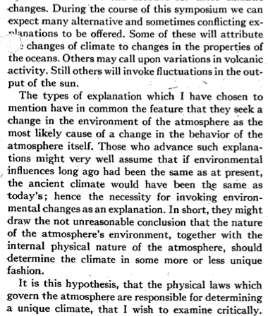
Here is Wentz & Schabel’s graph of IWV over time (shown as W in their figure):

From Wentz & Schabel (2000)

Figure 1 – Region captions added to each graph

They calculate, for the short period in question (1988-1998):

• 1.9%/decade for 20°N – 60°N
• 2.1%/decade for 20°S – 20°N
• 1.0%/decade for 20°S – 60°S

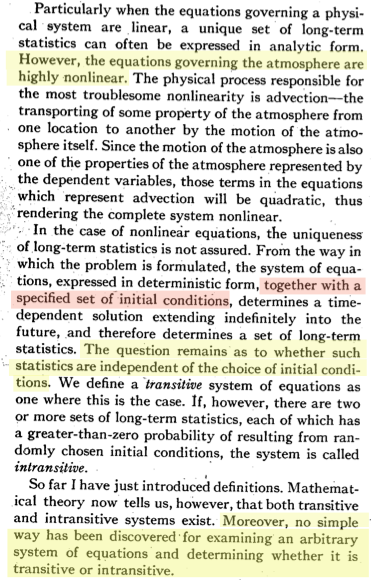
Soden et al (2005) take the dataset a little further and compare it to model results:

From Soden et al (2005)

Figure 2

They note the global trend of 1.4 ± 0.78 %/decade.

As their paper is more about upper tropospheric water vapor they also evaluate the change in channel 12 of the HIRS instrument (High Resolution Infrared Radiometer Sounder):

The radiance channel centered at 6.7 μm (channel 12) is sensitive to water vapor integrated over a broad layer of the upper troposphere (200 to 500 hPa) and has been widely used for studies of upper tropospheric water vapor. Because clouds strongly attenuate the infrared radiation, we restrict our analysis to clear-sky radiances in which the upwelling radiation in channel 12 is not affected by clouds.

The change in radiance from channel 12 is approximately zero over the time period, which for technical reasons (see note 1) corresponds to roughly constant relative humidity in that region over the period from the early 1980’s to 2004. You can read the technical explanation in their paper, but as we are focusing on total water vapor (IWV) we will leave a discussion over UTWV for another day.

Updated Radiosonde Trends

Durre et al (2009) updated radiosonde trends in their 2009 paper. There is a lengthy extract from the paper in note 2 (end of article) to give insight into why radiosonde data cannot just be taken “as is”, and why a method has to be followed to identify and remove stations with documented or undocumented instrument changes.

Importantly they note, as with Ross & Elliott 2001:

..Even though the stations were located in many parts of the globe, only a handful of those that qualified for the computation of trends were located in the Southern Hemisphere. Consequently, the trend analysis itself was restricted to the Northern Hemisphere as in that of RE01..

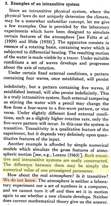
Here are their time-based trends:

From Durre et al (2009)

Figure 3

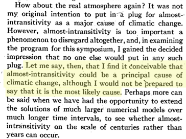
And a map of trends:

From Durre et al (2009)

Figure 4

Note the sparse coverage of the oceans and also the land regions in Africa and Asia, except China.

And their table of results:

From Durre et al (2009)

Figure 5

A very interesting note on the effect of their removal of stations based on detection of instrument changes and other inhomogeneities:

Compared to trends based on unadjusted PW data (not shown), the trends in Table 2 are somewhat more positive. For the Northern Hemisphere as a whole, the unadjusted trend is 0.22 mm/decade
, or 0.23 mm/decade
less than the adjusted trend.

This tendency for the adjustments to yield larger increases in PW is consistent with the notion that improvements in humidity measurements and observing practices over time have introduced an artificial drying into the radiosonde record (e.g., RE01).

TOPEX Microwave

Brown et al (2007) evaluated data from the Topex Microwave Radiometer (TMR). This is included on the Topex/Poseiden oceanography satellite and is dedicated to measuring the integrated water vapor content of the atmosphere. TMR is nadir pointing and measures the radiometric brightness temperature at 18, 21 and 37 GHz. As with SSMI, it only provides data over the ocean.

For the period of operation of the satellite (1992 – 2005) they found the trend of 0.90 ± 0.06 mm/decade:

From Brown et al (2007)

Figure 6 – Click for a slightly larger view

And a map view:

From Brown et al (2007)

Figure 7

Paltridge et al (2009)

Paltridge, Arking & Pook (2009) – P09 – take a look at the NCEP/NCAR reanalysis project from 1973 – 2007. They chose 1973 as the start date for the reasons explained in Part One – Elliott & Gaffen have shown that pre-1973 data has too many problems. They focus on humidity data below 500mbar as the measurement of humidity at higher altitudes and lower temperatures are more prone to radiosonde problems.

The NCEP/NCAR data shows positive trends below 850 mbar (=hPa) in all regions, negative trends above 850 mbar in the tropics and midlatitudes, and negative trends above 600 mbar in the northern midlatitudes.

Here are the water vapor trends vs height (pressure) for both relative humidity and specific humidity:

From Paltridge et al (2009)

Figure 8

And here is the map of trends:

from Paltridge et al (2009)

Figure 9

They comment on the “boundary layer” vs “free troposphere” issue.. In brief the boundary layer is that “well-mixed layer” close to the surface where the friction from the ground slows down the atmospheric winds and results in more turbulence and therefore a well-mixed layer of atmosphere. This is typically around 300m to 1000m high (there is no sharp “cut off”). At the ocean surface the atmosphere tends to be saturated (if the air is still) and so higher temperatures lead to higher specific humidities. (See Clouds and Water Vapor – Part Two if this is a new idea). Therefore, the boundary layer is uncontroversially expected to increase its water vapor content with temperature increases. It is the “free troposphere” or atmosphere above the boundary layer where the debate lies.

They comment:

It is of course possible that the observed humidity trends from the NCEP data are simply the result of problems with the instrumentation and operation of the global radiosonde network from which the data are derived.

The potential for such problems needs to be examined in detail in an effort rather similar to the effort now devoted to abstracting real surface temperature trends from the face-value data from individual stations of the international meteorological networks.

In the meantime, it is important that the trends of water vapor shown by the NCEP data for the middle and upper troposphere should not be “written off” simply on the basis that they are not supported by climate models—or indeed on the basis that they are not supported by the few relevant satellite measurements.

There are still many problems associated with satellite retrieval of the humidity information pertaining to a particular level of the atmosphere— particularly in the upper troposphere. Basically, this is because an individual radiometric measurement is a complicated function not only of temperature and humidity (and perhaps of cloud cover because “cloud clearing” algorithms are not perfect), but is also a function of the vertical distribution of those variables over considerable depths of atmosphere. It is difficult to assign a trend in such measurements to an individual cause.

Since balloon data is the only alternative source of information on the past behavior of the middle and upper tropospheric humidity and since that behavior is the dominant control on water vapor feedback, it is important that as much information as possible be retrieved from within the “noise” of the potential errors.

So what has P09 added to the sum of knowledge? We can already see the NCEP/NCAR trends in Trends and variability in column-integrated atmospheric water vapor by Trenberth et al from 2005.

Did the authors just want to take the reanalysis out of the garage, drive it around the block a few times and park it out front where everyone can see it?

No, of course not!

– I hear all the NCEP/NCAR believers say.

One of our commenters asked me to comment on Paltridge’s reply to Dessler (which was a response to Paltridge..), and linked to another blog article. It seems like even the author of that blog article is confused about NCEP/NCAR. This reanalysis project (as explained in Part One), is a model output not a radiosonde dataset:

Humidity is in category B – ‘although there are observational data that directly affect the value of the variable, the model also has a very strong influence on the value ‘

And for those people who have a read of Kalnay’s 1996 paper describing the project they will see that with the huge amount of data going into the model, the data wasn’t quality checked by human inspection on the way in. Various quality control algorithms attempt to (automatically) remove “bad data”.

This is why we have reviewed Ross & Elliott (2001) and Durre et al (2009). These papers review the actual radiosonde data and find increasing trends in IWV. They also describe in a lot of detail what kind of process they had to go through to produce a decent dataset. The authors of both papers also both explained that they could only produce a meaningful trend for the northern hemisphere. There is not enough quality data for the southern hemisphere to even attempt to produce a trend.

And Durre et al note that when they use the complete dataset the trend is half that calculated with problematic data removed.

This is the essence of the problem with Paltridge et al (2009)

Why is Ross & Elliot (2001) not reviewed and compared? If Ross & Elliott found that Southern Hemisphere trends could not be calculated because of the sparsity of quality radiosonde data, why doesn’t P09 comment on that? Perhaps Ross & Elliott are wrong. But no comment from P09. (Durre et al find the same problem with SH data, and probably too late for P09 but not too late for the 2010 comments the authors have been making).

In The Mass of the Atmosphere: A Constraint on Global Analyses, Trenberth & Smith pointed out clear problems with NCEP/NCAR vs ERA-40. Perhaps Trenberth and Smith are wrong. Or perhaps there is another way to understand these results. But no comment on this from P09.

P09 comment on the issues with satellite humidity retrieval for different layers of the atmosphere but no comment on the results from the microwave SSMI which has a totally different algorithm to retrieve IWV. And it is important to understand that they haven’t actually demonstrated a problem with satellite measurements. Let’s review their comment:

In the meantime, it is important that the trends of water vapor shown by the NCEP data for the middle and upper troposphere should not be “written off” simply on the basis that they are not supported by climate models—or indeed on the basis that they are not supported by the few relevant satellite measurements.

The reader of the paper wouldn’t know that Trenberth & Smith have demonstrated an actual reason for preferring ERA-40 (if any reanalysis is to be used).

The reader of the paper might understand “a few relevant satellite measurements” as meaning there wasn’t much data from satellites. If you review figure 4 you can see that the quality radiosonde data is essentially mid-latitude northern hemisphere land. Satellites – that is, multiple satellites with different instruments at different frequencies – have covered the oceans much much more comprehensively than radiosondes. Are the satellites all wrong?

The reader of the paper would think that the dataset has been apparently ditched because it doesn’t fit climate models.

This is probably the view of Paltridge, Arking & Pook. But they haven’t demonstrated it. They have just implied it.

Dessler & Davis (2010)

Dessler & Davis responded to P09. They plot some graphs from 1979  to present. The reason for plotting graphs from 1979 is because this is when the satellite data was introduced. And all of the reanalysis projects, except NCEP/NCAR incorporated satellite humidity data. (NCEP/NCAR does incorporate satellite data for some other fields).

Basically when data from a new source is introduced, even if it is more accurate, it can introduce spurious trends and even in opposite direction to the real trends. This was explained in Part One under the heading Comparing Reanalysis of Humidity. So trend analysis usually takes place over periods of consistent data sources.

This figure contrasts short term relationships between temperature and humidity with long term relationships:

From Dessler & Davis (2010)

Figure 10

If the blog I referenced earlier is anything to go by, the primary reason for producing this figure has been missed. And as that blog article seemed to not comprehend that NCEP/NCAR is a reanalysis (= model output) it’s not so surprising.

Dessler & Davis said:

There is poorer agreement among the reanalyses, particularly compared to the excellent agreement for short‐term fluctuations. This makes sense: handling data inhomogeneities will introduce long‐term trends in the data but have less effect on short‐term trends. This is why long term trends from reanalyses tend to be looked at with suspicion [e.g., Paltridge et al., 2009; Thorne and Vose, 2010; Bengtsson et al., 2004].

[Emphasis added]

They are talking about artifacts of the model (NCEP/NCAR). In the short term the relationship between humidity and temperature agree quite well among the different reanalyses. But in the longer term NCEP/NCAR doesn’t – demonstrating that it is likely introducing biases.

The alternative, as Dessler & Davis explain, is that there is somehow an explanation for a long term negative feedback (temperature and water vapor) with a short term positive feedback.

If you look around the blog world, or at say, Professor Lindzen you don’t find this. You find arguments about why short term feedback is negative. Not an argument that short term is positive and yet long term is negative.

I agree that many people say:  “I don’t know, it’s complicated, perhaps there is a long term negative feedback..” and I respect that point of view.

But in the blog article pointed to me by our commenter in Part One, the author said:

JGR let some decidedly unscientific things slip into that Dessler paper. One of the reasons provided is nothing more than a form of argument from ignorance: “there’s no theory that explains why the short term might be different to the long term”.

Why would any serious scientist admit that they don’t have the creativity or knowledge to come up with some reasons, and worse, why would they think we’d find that ignorance convincing?

..It’s not that difficult to think of reasons why it’s possible that humidity might rise in the short run, but then circulation patterns or other slower compensatory effects shift and the long run pattern is different. Indeed they didn’t even have to look further than the Paltridge paper they were supposedly trying to rebut (see Garth’s writing below). In any case, even if someone couldn’t think of a mechanism in a complex unknown system like our climate, that’s not “a reason” worth mentioning in a scientific paper.

The point that seems to have been missed is this is not a reason to ditch the primary dataset but instead a reason why NCEP/NCAR is probably flawed compared with all the other reanalyses. And compared with the primary dataset. And compared with multiple satellite datasets.

This is the issue with reanalyses. They introduce spurious biases. Bengsston explained how (specifically for ERA-40). Trenberth & Smith have already demonstrated it for NCEP/NCAR. And now Dessler & Davis have simply pointed out another reason for taking that point of view.

The blog writer thinks that Dessler is trying to ditch the primary dataset because of an argument from ignorance. I can understand the confusion.

It is still confusion.

One last point to add is that Dessler & Davis also added the very latest in satellite water vapor data – the AIRS instrument from 2003. AIRS is a big step forward in satellite measurement of water vapor, a subject for another day.

AIRS also shows the same trends as the other reanalyses and different from NCEP/NCAR.

A Scenario

Before reaching the conclusion I want to throw a scenario out there. It is imaginary.

Suppose that there were two sources of data for temperature over the surface of the earth – temperature stations and satellite. Suppose the temperature stations were located mainly in mid-latitude northern hemisphere locations. Suppose that there were lots of problems with temperature stations – instrument changes & environmental changes close to the temperature stations (we will call these environmental changes “UHI”).

Suppose the people who had done the most work analyzing the datasets and trying to weed out the real temperature changes from the spurious ones had demonstrated that the temperature had decreased over northern hemisphere mid-latitudes. And that they had claimed that quality southern hemisphere data was too “thin on the ground” to really draw any conclusions from.

Suppose that satellite data from multiple instruments, each using different technology, had also demonstrated that temperatures were decreasing over the oceans.

Suppose that someone fed the data from the (mostly NH) land-based temperature stations – without any human intervention on the UHI and instrument changes – into a computer model.

And suppose this computer model said that temperatures were increasing.

Imagine it, for a minute. I think we can picture the response.

And yet, this is a similar situation that we are confronted with on integrated water vapor (IWV). I have tried to think of a reason why so many people would be huge fans of this particular model output. I did think of one, but had to reject it immediately as being ridiculous.

I hope someone can explain why NCEP/NCAR deserves the fan club it has currently built up.

Conclusion

Radiosonde datasets, despite their problems, have been analyzed. The researchers have found positive water vapor trends for the northern hemisphere with these datasets. As far as I know, no one has used radiosonde datasets to find the opposite.

Radiosonde datasets provide excellent coverage for mid-latitude northern hemisphere land, and, with a few exceptions, poor coverage elsewhere.

Satellites, using IR and microwave, demonstrate increasing water vapor over the oceans for the shorter time periods in which they have been operating.

Reanalysis projects have taken in various data sources and, using models, have produced output values for IWV (total water vapor) with mixed results.

Reanalysis projects all have the benefit of convenience, but none are perfect. The dry mass of the atmosphere, which should be constant within noise errors unless a new theory comes along, demonstrates that NCEP/NCAR is worse than ERA-40.

ERA-40 demonstrates increasing IWV. NCEP/NCAP demonstrates negative IWV.

Some people have taken NCEP/NCAR for a drive around the block and parked it in front of their house and many people have wandered down the street to admire it. But it’s not the data. It’s a model.

Perhaps Paltridge, Arking or Pook can explain why NCEP/NCAR is a quality dataset. Unfortunately, their paper doesn’t demonstrate it.

It seems that some people are really happy if one model output or one dataset or one paper says something different from what 5 or 10 or 100 others are saying. If that makes you, the reader, happy, then at least the world has less deaths from stress.

In any field of science there are outliers.

The question on this blog at least, is what can be proven, what can be demonstrated and what evidence lies behind any given claim. From this blog’s perspective, the fact that outliers exist isn’t really very interesting. It is only interesting to find out if in fact they have merit.

In the world of historical climate datasets nothing is perfect. It seems pretty clear that integrated water vapor has been increasing over the last 20-30 years. But without satellites, even though we have a long history of radiosonde data, we have quite a limited dataset geographically.

If we can only use radiosonde data perhaps we can just say that water vapor has been increasing over northern hemisphere mid-latitude land for nearly 40 years. If we can use satellite as well, perhaps we can say that water vapor has been increasing everywhere for over 20 years.

If we can use the output from reanalysis models and do a lucky dip perhaps we can get a different answer.

And if someone comes along, analyzes the real data and provides a new perspective then we can all have another review.

References

On the Utility of Radiosonde Humidity Archives for Climate Studies, Elliot & Gaffen, Bulletin of the American Meteorological Society (1991)

Relationships between Tropospheric Water Vapor and Surface Temperature as Observed by Radiosondes, Gaffen, Elliott & Robock, Geophysical Research Letters(1992)

Column Water Vapor Content in Clear and Cloudy Skies, Gaffen & Elliott, Journal of Climate (1993)

On Detecting Long Term Changes in Atmospheric Moisture, Elliot, Climate Change (1995)

Tropospheric Water Vapor Climatology and Trends over North America, 1973-1993, Ross & Elliot, Journal of Climate (1996)

An assessment of satellite and radiosonde climatologies of upper-tropospheric water vapor, Soden & Lanzante, Journal of Climate (1996)

The NCEP/NCAR 40-year Reanalysis Project, Kalnay et al, Bulletin of the American Meteorological Society (1996)

Precise climate monitoring using complementary satellite data sets, Wentz & Schabel, Nature (2000)

Radiosonde-Based Northern Hemisphere Tropospheric Water Vapor Trends, Ross & Elliott, Journal of Climate (2001)

An analysis of satellite, radiosonde, and lidar observations of upper tropospheric water vapor from the Atmospheric Radiation Measurement Program, Soden et al,  Journal of Geophysical Research (2005)

The Radiative Signature of Upper Tropospheric Moistening, Soden et al, Science (2005)

The Mass of the Atmosphere: A Constraint on Global Analyses, Trenberth & Smith, Journal of Climate (2005)

Trends and variability in column-integrated atmospheric water vapor, Trenberth et al, Climate Dynamics (2005)

Can climate trends be calculated from reanalysis data? Bengtsson et al, Journal of Geophysical Research (2005)

Ocean Water Vapor and Cloud Burden Trends Derived from the Topex Microwave Radiometer, Brown et al, Geoscience and Remote Sensing Symposium, 2007. IGARSS 2007. IEEE International (2007)

Radiosonde-based trends in precipitable water over the Northern Hemisphere: An update, Durre et al, Journal of Geophysical Research (2009)

Trends in middle- and upper-level tropospheric humidity from NCEP reanalysis data, Paltridge et al, Theoretical Applied Climatology (2009)

Trends in tropospheric humidity from reanalysis systems, Dessler & Davis, Journal of Geophysical Research (2010)

Notes

Note 1: The radiance measurement in this channel is a result of both the temperature of the atmosphere and the amount of water vapor. If temperature increases radiance increases. If water vapor increases it attenuates the radiance. See the slightly more detailed explanation in their paper.

Note 2: Here is a lengthy extract from Durre et al (2009), partly because it’s not available for free, and especially to give an idea of the issues arising from trying to extract long term climatology from radiosonde data and, therefore, careful approach that needs to be taken.

Emphasis added in each case:

From the IGRA+RE01 data, stations were chosen on the basis of two sets of requirements: (1) criteria that qualified them for use in the homogenization process and (2) temporal completeness requirements for the trend analysis.

In order to be a candidate for homogenization, a 0000 UTC or 1200 UTC time series needed to both contain at least two monthly means in each of the 12 calendar months during 1973–2006 and have at least five qualifying neighbors (see section 2.2). Once adjusted, each time series was tested against temporal completeness requirements analogous to those used by RE01; it was considered sufficiently complete for the calculation of a trend if it contained no more than 60 missing months, and no data gap was longer than 36 consecutive months.

Approximately 700 stations were processed through the pairwise homogenization algorithm (hereinafter abbreviated as PHA) at each of the nominal observation times. Even though the stations were located in many parts of the globe, only a handful of those that qualified for the computation of trends were located in the Southern Hemisphere.

Consequently, the trend analysis itself was restricted to the Northern Hemisphere as in that of RE01. The 305 Northern Hemisphere stations for 0000 UTC and 280 for 1200 UTC that fulfilled the completeness requirements covered mostly North America, Greenland, Europe, Russia, China, and Japan.

Compared to RE01, the number of stations for which trends were computed increased by more than 100, and coverage was enhanced over Greenland, Japan, and parts of interior Asia. The larger number of qualifying
stations was the result of our ability to include stations that were sufficiently complete but contained significant inhomogeneities that required adjustment.

Considering that information on these types of changes tends to be incomplete for the historical record, the successful adjustment for inhomogeneities requires an objective technique that not only uses any available metadata, but also identifies undocumented change points [Gaffen et al., 2000; Durre et al., 2005]. The PHA of MW09 has these capabilities and thus was used here. Although originally developed for homogenizing time series of monthly mean surface temperature, this neighbor-based procedure was designed such that it can be applied to other variables, recognizing that its effectiveness depends on the relative magnitudes of change points compared to the spatial and temporal variability of the variable.

As can be seen from Table 1, change points were identified in 56% of the 0000 UTC and 52% of the 1200 UTC records, for a total of 509 change points in 317 time series.

Of these, 42% occurred around the time of a known metadata event, while the remaining 58% were considered to be ‘‘undocumented’’ relative to the IGRA station history information. On the basis of the visual inspection, it appears that the PHA has a 96% success rate at detecting obvious discontinuities. The algorithm can be effective even when a particular step change is present at the target and a number of its neighbors simultaneously.

In Japan, for instance, a significant drop in PW associated with a change between Meisei radiosondes around 1981 (Figure 1, top) was detected in 16 out of 17 cases, thanks to the inclusion of stations from adjacent tries in the pairwise comparisons Furthermore, when an adjustment is made around the time of a documented change in radiosonde type, its sign tends to agree with that expected from the known biases of the relevant instruments. For example, the decrease in PW at Yap in 1995 (Figure 1, middle) is consistent with the artificial drying expected from the change from a VIZ B to a Vaisala RS80–56 radiosonde that is known to have occurred at this location and time [Elliott et al., 2002; Wang and Zhang, 2008].

Read Full Post »

Water vapor trends is a big subject and so this article is not a comprehensive review – there are a few hundred papers on this subject. However, as most people outside of climate scientists have exposure to blogs where only a few papers have been highlighted, perhaps it will help to provide some additional perspective.

Think of it as an article that opens up some aspects of the subject.

And I recommend reading a few of the papers in the References section below. Most are linked to a free copy of the paper.

Mostly what we will look at in this article is “total precipitable water vapor” (TPW) also known as “column integrated water vapor (IWV)”.

What is this exactly? If we took a 1 m² area at the surface of the earth and then condensed the water vapor all the way up through the atmosphere, what height would it fill in a 1 m² tub?

The average depth (in this tub) from all around the world would be about 2.5 cm. Near the equator the amount would be 5cm and near the poles it would be 0.5 cm.

Averaged globally, about half of this is between sea level and 850 mbar (around 1.5 km above sea level), and only about 5% is above 500 mbar (around 5-6 km above sea level).

Where Does the Data Come From?

How do we find IVW (integrated water vapor)?

• Radiosondes
• Satellites

Frequent radiosonde launches were started after the Second World War – prior to that knowledge of water vapor profiles through the atmosphere is very limited.

Satellite studies of water vapor did not start until the late 1970’s.

Unfortunately for climate studies, radiosondes were designed for weather forecasting and so long term trends were not a factor in the overall system design.

Radiosondes were mostly launched over land and are predominantly from the northern hemisphere.

Given that water vapor response to climate is believed to be mostly from the ocean (the source of water vapor), not having significant measurements over the ocean until satellites in the late 1970’s is a major problem.

There is one more answer that could be added to the above list:

• Reanalyses

As most people might suspect from the name, a reanalysis isn’t a data source. We will take a look at them a little later.

Quick List

Pros and Cons in brief:

Radiosonde Pluses:

• Long history
• Good vertical resolution
• Can measure below clouds

Radiosonde Minuses:

• Geographically concentrated over northern hemisphere land
• Don’t measure low temperature or low humidity reliably
• Changes to radiosonde sensors and radiosonde algorithms have subtly (or obviously) changed the measured values

Satellite Pluses:

• Global coverage
• Consistency of measurement globally and temporally
• Changes in satellite sensors can be more easily checked with inter-comparison tests

Satellite Minuses:

• Shorter history (since late 1970’s)
• Vertical resolution of a few kms rather than hundreds of meters
• Can’t measure under clouds (limit depends on whether infrared or microwave is used)
• Requires knowledge of temperature profile to convert measured radiances to humidity

Radiosonde Measurements

Three names that come up a lot in papers on radiosonde measurements are Gaffen, Elliott and Ross. Usually pairing up they have provided a some excellent work on radiosonde data and on measurement issues with radiosondes.

From Radiosonde-based Northern Hemisphere Tropospheric Water Vapor Trends, Ross & Elliott (2001):

All the above trend studies considered the homogeneity of the time series in the selection of stations and the choice of data period. Homogeneity of a record can be affected by changes in instrumentation or observing practice. For example, since relative humidity typically decreases with height through the atmosphere, a fast responding humidity sensor would report a lower relative humidity than one with a greater lag in response.

Thus, the change to faster-response humidity sensors at many stations over the last 20 years could produce an apparent, though artificial, drying over time..

Then they have a section discussing various data homogeneity issues, which includes this graphic showing the challenge of identifying instrument changes which affect measurements:

From Ross & Elliott (2001)

Figure 1

They comment:

These examples show that the combination of historical and statistical information can identify some known instrument changes. However, we caution that the separation of artificial (e.g., instrument changes) and natural variability is inevitably somewhat subjective. For instance, the same instrument change at one station may not show as large an effect at another location or time of day..

Furthermore, the ability of the statistical method to detect abrupt changes depends on the variability of the record, so that the same effect of an instrument change could be obscured in a very noisy record. In this case, the same change detected at one station may not be detected at another station containing more variability.

Here are their results from 1973-1995 in geographical form. Triangles are positive trends, circles are negative trends. You also get to see the distribution of radiosondes, as each marker indicates one station:

Figure 2

And their summary of time-based trends for each region:

Figure 3

In their summary they make some interesting comments:

We found that a global estimate could not be made because reliable records from the Southern Hemisphere were too sparse; thus we confined our analysis to the Northern Hemisphere. Even there, the analysis was limited by continual changes in instrumentation, albeit improvements, so we were left with relatively few records of total precipitable water over the era of radiosonde observations that were usable.

Emphasis added.

Well, I recommend that readers take the time to read the whole paper for themselves to understand the quality of work that has been done – and learn more about the issues with the available data.

What is Special about 1973?

In their 1991 paper, Elliot and Gaffen showed that pre-1973 radiosonde measurements came with much more problems than post-1973.

From Elliott & Gaffen (1991)

Figure 4 – Click for larger view

Note that the above is just for the US radiosonde network.

 Our findings suggest caution is appropriate when using the humidity archives or interpreting existing water vapor climatologies so that changes in climate not be confounded by non-climate changes.

And one extract to give a flavor of the whole paper:

The introduction of the new hygristor in 1980 necessitated a new algorithm.. However, the new algorithm also eliminated the possibility of reports of humidities greater than 100% but ensured that humidities of 100% cannot be reported in cold temperatures. The overall effect of these changes is difficult to ascertain. The new algorithm should have led to higher reported humidities compared to the older algorithm, but the elimination of reports of very high values at cold temperatures would act in the opposite sense.

And a nice example of another change in radiosonde measurement and reporting practice. The change below is just an artifact of low humidity values being reported after a certain date:

From Elliott & Gaffen (1991)

Figure 5

As the worst cases came before 1973, most researchers subsequently reporting on water vapor trends have tended to stick to post-1973 (or report on that separately and add caveats to pre-1973 trends).

But it is important to understand that issues with radiosonde measurements are not confined to pre-1973.

Here are a few more comments, this time from Elliott in his 1995 paper:

Most (but not all) of these changes represent improvements in sensors or other practices and so are to be welcomed. Nevertheless they make it difficult to separate climate changes from changes in the measurement programs..

Since then, there have been several generations of sensors and now sensors have much faster response times. Whatever the improvements for weather forecasting, they do leave the climatologist with problems. Because relative humidity generally decreases with height slower sensors would indicate a higher humidity at a given height than today’s versions (Elliott et al., 1994).

This effect would be particularly noticeable at low temperatures where the differences in lag are greatest. A study by Soden and Lanzante (submitted) finds a moist bias in upper troposphere radiosondes using slower responding humidity sensors relative to more rapid sensors, which supports this conjecture. Such improvements would lead the unwary to conclude that some part of the atmosphere had dried over the years.

And Gaffen, Elliott & Robock (1992) reported that in analyzing data from 50 stations from 1973-1990 they found instrument changes that created “inhomogeneities in the records of about half the stations”

Satellite Demonstration

Different countries tend to use different radiosondes, have different algorithms and have different reporting practices in place.

The following comparison is of upper tropospheric water vapor. As an aside this has a focus because water vapor in the upper atmosphere disproportionately affects top of atmosphere radiation – and therefore the radiation balance of the climate.

From Soden & Lanzante (1996), the data below, of the difference between satellite and radiosonde measurements, identifies a significant problem:

Soden & Lanzante (1996)

Figure 6

Since the same satellite is used in the comparison at all radiosonde locations, the satellite measurements serve as a fixed but not absolute reference. Thus we can infer that radiosonde values over the former Soviet Union tend to be systematically moister than the satellite measurements, that are in turn systematically moister than radiosonde values over western Europe.

However, it is not obvious from these data which of the three sets of measurements is correct in an absolute sense. That is, all three measurements could be in error with respect to the actual atmosphere..

..However, such a satellite [calibration] error would introduce a systematic bias at all locations and would not be regionally dependent like the bias shown in fig. 3 [=figure 6].

They go on to identify the radiosonde sensor used in different locations as the likely culprit. Yet, as various scientists comment in their papers, countries take on a new radiosonde in piecemeal form, sometimes having a “competitive supply” situation where 70% is from one vendor and 30% from another vendor. Other times radiosonde sensors are changed across a region over a period of a few years. Inter-comparisons are done, but inadequately.

Soden and Lanzante also comment on spatial coverage:

Over data-sparse regions such as the tropics, the limited spatial coverage can introduce systematic errors of 10-20% in terms of the relative humidity. This problem is particularly severe in the eastern tropical Pacific, which is largely void of any radiosonde stations yet is especially critical for monitoring interannual variability (e.g. ENSO).

Before we move onto reanalyses, a summing up on radiosondes from the cautious William P. Elliot (1995):

Thus there is some observational evidence for increases in moisture content in the troposphere and perhaps in the stratosphere over the last 2 decades. Because of limitations of the data sources and the relatively short record length, further observations and careful treatment of existing data will be needed to confirm a global increase.

Reanalysis – or Filling in the Blanks

Weather forecasting and climate modelling is a form of finite element analysis (and see Wikipedia). Essentially in FEA, some kind of grid is created – like this one for a pump impellor:

Stress analysis in an impeller

Figure 7

– and the relevant equations can be solved for each boundary or each element. It’s a numerical solution to a problem that can’t be solved analytically.

Weather forecasting and climate are as tough as they come. Anyway, the atmosphere is divided up into a grid and in each grid we need a value for temperature, pressure, humidity and many other variables.

To calculate what the weather will be like over the next week a value needs to be placed into each and every grid. And just one value. If there is no value in the grid the program can’t run and there’s nowhere to put two values.

By this massive over-simplification, hopefully you will be able to appreciate what a reanalysis does. If no data is available, it has to be created. That’s not so terrible, so long as you realize it:

Figure 8

This is a simple example where the values represent temperatures in °C as we go up through the atmosphere. The first problem is that there is a missing value. It’s not so difficult to see that some formula can be created which will give a realistic value for this missing value. Perhaps the average of all the values surrounding it? Perhaps a similar calculation which includes values further away, but with less weighting.

With some more meteorological knowledge we might develop a more sophisticated algorithm based on the expected physics.

The second problem is that we have an anomaly. Clearly the -50°C is not correct. So there needs to be an algorithm which “fixes” it. Exactly what fix to use presents the problem.

If data becomes sparser then the problems get starker. How do we fill in and correct these values?

Figure 9

It’s not at all impossible. It is done with a model. Perhaps we know surface temperature and the typical temperature profile (“lapse rate”) through the atmosphere. So the model fills in the blanks with “typical climatology” or “basic physics”.

But it is invented data. Not real data.

Even real data is subject to being changed by the model..

NCEP/NCAR Reanalysis Project

There are a number of reanalysis projects. One is the NCEP/NCAR project (NCEP = National Centers for Environmental Prediction, NCAR = National Center for Atmospheric Research).

Kalnay (1996) explains:

The basic idea of the reanalysis project is to use a frozen state-of-the-art analysis/forecast system and perform data assimilation using past data, from 1957 to the present (reanalysis).

The NCEP/NCAR 40-year reanalysis project should be a research quality dataset suitable for many uses, including weather and short-term climate research.

An important consideration is explained:

An important question that has repeatedly arisen is how to handle the inevitable changes in the observing system, especially the availability of new satellite data, which will undoubtedly have an impact on the perceived climate of the reanalysis. Basically the choices are a) to select a subset of the observations that remains stable throughout the 40-year period of the reanalysis, or b) to use all the available data at a given time.

Choice a) would lead to an reanalysis with the most stable climate, and choice b) to an analysis that is as accurate as possible throughout the 40 years. With the guidance of the advisory panel, we have chosen b), that is, to make use of the most data available at any given time.

What are the categories of output data?

• A = analysis variable is strongly influenced by observed data and hence it is in the most reliable class
• B = although there are observational data that directly affect the value of the variable, the model also has a very strong influence on the value
• C = there are no observations directly affecting the variable, so that it is derived solely from the model fields

Humidity is in category B.

Interested people can read Kalnay’s paper. Reanalysis products are very handy and widely used. Those with experience usually know what they are playing around with. Newcomers need to pay attention to the warning labels.

Comparing Reanalysis of Humidity

Bengtsson et al (2004) reviewed another reanalysis project, ERA-40. They provide a good example of how incorrect trends can be introduced (especially the 2nd paragraph):

A bias changing in time can thus introduce a fictitious trend without being eliminated by the data assimilation system. A fictitious trend can be generated by the introduction of new types of observations such as from satellites and by instrumental and processing changes in general. Fictitious trends could also result from increases in observational coverage since this will affect systematic model errors.

Assume, for example, that the assimilating model has a cold bias in the upper troposphere which is a common error in many general circulation models (GCM). As the number of observations increases the weight of the model in the analysis is reduced and the bias will correspondingly become smaller. This will then result in an artificial warming trend.

Bengtsson and his colleagues analyze tropospheric temperature, IWV and kinetic energy.

ERA-40 does have a positive trend in water vapor, something we will return to. The trend from ERA-40 for 1958-2001 is +0.41 mm/decade, and for 1979-2001 = +0.36 mm/decade. They note that NCEP/NCAR has a negative trend of -0.24 mm/decade from 1958-2001 and -0.06mm/decade  for 1979-2001, but it isn’t a focus of their study.

They do an analysis which excludes satellite data and find a lower (but still positive) trend for IWV. They also question the magnitudes of tropospheric temperature trends and kinetic energy on similar grounds.

The point is essentially that the new data has created a bias in the reanalysis.

Their conclusion, following various caveats about the scale of the study so far:

Returning finally to the question in the title of this study an affirmative answer cannot be given, as the indications are that in its present form the ERA40 analyses are not suitable for long-term climate trend calculations.

However, it is believed that there are ways forward as indicated in this study which in the longer term are likely to be successful. The study also stresses the difficulties in detecting long term trends in the atmosphere and major efforts along the lines indicated here are urgently needed.

So, onto Trends and variability in column-integrated atmospheric water vapor by Trenberth, Fasullo & Smith (2005). This paper is well worth reading in full.

For years before 1996, the Ross and Elliott radiosonde dataset is used for validation of European Centre for Medium-range Weather Forecasts (ECMWF) reanalyses ERA-40. Only the special sensor microwave imager (SSM/I) dataset from remote sensing systems (RSS) has credible means, variability and trends for the oceans, but it is available only for the post-1988 period.

Major problems are found in the means, variability and trends from 1988 to 2001 for both reanalyses from National Centers for Environmental Prediction (NCEP) and the ERA-40 reanalysis over the oceans, and for the NASA water vapor project (NVAP) dataset more generally. NCEP and ERA-40 values are reasonable over land where constrained by radiosondes.

Accordingly, users of these data should take great care in accepting results as real.

Here’s a comparison of Ross & Elliott (2001) [already shown above] with ERA-40:

From Trenberth et al (2005)

Figure 10 – Click for a larger image

Then they consider 1988-2001, the reason being that 1988 was when the SSMI (special sensor microwave imager) data over the oceans became available (more on the satellite data later).

From Trenberth et al (2005)

Figure 11

At this point we can see that ERA-40 agrees quite well with SSMI (over the oceans, the only place where SSMI operates), but NCEP/NCAR and another reanalysis product, NVAR, produce flat trends.

Now we will take a look at a very interesting paper: The Mass of the Atmosphere: A Constraint on Global Analyses, Trenberth & Smith (2005). Most readers will probably not be aware of this comparison and so it is of “extra” interest.

The total mass of the atmosphere is in fact a fundamental quantity for all atmospheric sciences. It varies in time because of changing constituents, the most notable of which is water vapor. The total mass is directly related to surface pressure while water vapor mixing ratio is measured independently.

Accordingly, there are two sources of information on the mean annual cycle of the total mass and the associated water vapor mass. One is from measurements of surface pressure over the globe; the other is from the measurements of water vapor in the atmosphere.

The main idea is that other atmospheric mass changes have a “noise level” effect on total mass, whereas water vapor has a significant effect. As measurement of surface pressure is a fundamental meteorological value, measured around the world continuously (or, at least, continually), we can calculate the total mass of the atmosphere with high accuracy. We can also – from measurements of IWV – calculate the total mass of water vapor “independently”.

Subtracting water vapor mass from total atmospheric measured mass should give us a constant – the “dry atmospheric pressure”. That’s the idea. So if we use the surface pressure and the water vapor values from various reanalysis products we might find out some interesting bits of data..

from Trenberth & Smith (2005)

Figure 12

In the top graph we see the annual cycle clearly revealed. The bottom graph is the one that should be constant for each reanalysis. This has water vapor mass removed via the values of water vapor in that reanalysis.

Pre-1973 values show up as being erratic in both NCEP and ERA-40. NCEP values show much more variability post-1979, but neither is perfect.

The focus of the paper is the mass of the atmosphere, but is still recommended reading.

Here is the geographical distribution of IWV and the differences between ERA-40 and other datasets (note that only the first graphic is trends, the following graphics are of differences between datasets):

Trenberth et al (2005)

Figure 13 – Click for a larger image

The authors comment:

The NCEP trends are more negative than others in most places, although the patterns appear related. Closer examination reveals that the main discrepancies are over the oceans. There is quite good agreement between ERA-40 and NCEP over most land areas except Africa, i.e. in areas where values are controlled by radiosondes.

There’s a lot more in the data analysis in the paper. Here are the trends from 1988 – 2001 from the various sources including ERA-40 and SSMI:

From Trenberth et al (2005)

Figure 14 – Click for a larger view

• SSMI has a trend of +0.37 mm/decade.
• ERA-40  has a trend of +0.70mm/decade over the oceans.
• NCEP has a trend of -0.1mm/decade over the oceans.

To be Continued..

As this article is already pretty long, it will be continued in Part Two, which will include Paltridge et al (2009), Dessler & Davis (2010) and some satellite measurements and papers.

Update – Part Two is published

References

On the Utility of Radiosonde Humidity Archives for Climate Studies, Elliot & Gaffen, Bulletin of the American Meteorological Society (1991)

Relationships between Tropospheric Water Vapor and Surface Temperature as Observed by Radiosondes, Gaffen, Elliott & Robock, Geophysical Research Letters (1992)

Column Water Vapor Content in Clear and Cloudy Skies, Gaffen & Elliott, Journal of Climate (1993)

On Detecting Long Term Changes in Atmospheric Moisture, Elliot, Climate Change (1995)

Tropospheric Water Vapor Climatology and Trends over North America, 1973-1993, Ross & Elliot, Journal of Climate (1996)

An assessment of satellite and radiosonde climatologies of upper-tropospheric water vapor, Soden & Lanzante, Journal of Climate (1996)

The NCEP/NCAR 40-year Reanalysis Project, Kalnay et al, Bulletin of the American Meteorological Society (1996)

Radiosonde-Based Northern Hemisphere Tropospheric Water Vapor Trends, Ross & Elliott, Journal of Climate (2001)

An analysis of satellite, radiosonde, and lidar observations of upper tropospheric water vapor from the Atmospheric Radiation Measurement Program, Soden et al,  Journal of Geophysical Research (2005)

The Radiative Signature of Upper Tropospheric Moistening, Soden et al, Science (2005)

The Mass of the Atmosphere: A Constraint on Global Analyses, Trenberth & Smith, Journal of Climate (2005)

Trends and variability in column-integrated atmospheric water vapor, Trenberth et al, Climate Dynamics (2005)

Can climate trends be calculated from reanalysis data? Bengtsson et al, Journal of Geophysical Research (2005)

Trends in middle- and upper-level tropospheric humidity from NCEP reanalysis data, Paltridge et al, Theoretical Applied Climatology (2009)

Trends in tropospheric humidity from reanalysis systems, Dessler & Davis, Journal of Geophysical Research (2010)

Read Full Post »