In Part Three – Attribution & Fingerprints we looked at an early paper in this field, from 1996. I was led there by following back through many papers referenced from AR5 Chapter 10. The lead author of that paper, Gabriele Hegerl, has made a significant contribution to the 3rd report, 4th and 5th IPCC reports on attribution.
We saw in Part Three that this particular paper ascribed a probability:
We find that the latest observed 30-year trend pattern of near-surface temperature change can be distinguished from all estimates of natural climate variability with an estimated risk of less than 2.5% if the optimal fingerprint is applied.
That paper did note that greatest uncertainty was in understanding the magnitude of natural variability. This is an essential element of attribution.
It wasn’t explicitly stated whether the 97.5% confidence was with the premise that natural variability was accurately understood in 1996. I believe that this was the premise. I don’t know what confidence would have been ascribed to the attribution study if uncertainty over natural variability was included.
IPCC AR5
In this article we will look at the IPCC 5th report, AR5, and see how this field has progressed, specifically in regard to the understanding of natural variability. Chapter 10 covers Detection and Attribution of Climate Change.
From p.881 (the page numbers are from the start of the whole report, chapter 10 has just over 60 pages plus references):
Since the AR4, detection and attribution studies have been carried out using new model simulations with more realistic forcings, and new observational data sets with improved representation of uncertainty (Christidis et al., 2010; Jones et al., 2011, 2013; Gillett et al., 2012, 2013; Stott and Jones, 2012; Knutson et al., 2013; Ribes and Terray, 2013).
Let’s have a look at these papers (see note 1 on CMIP3 & CMIP5).
I had trouble understanding AR5 Chapter 10 because there was no explicit discussion of natural variability. The papers referenced (usually) have their own section on natural variability, but chapter 10 doesn’t actually cover it.
I emailed Geert Jan van Oldenborgh to ask for help. He is the author of one paper we will briefly look at here – his paper was very interesting and he had a video segment explaining his paper. He suggested the problem was more about communication because natural variability was covered in chapter 9 on models. He had written a section in chapter 11 that he pointed me towards, so this article became something that tried to grasp the essence of three chapters (9 – 11), over 200 pages of reports and several pallet loads of papers.
So I’m not sure I can do the synthesis justice, but what I will endeavor to do in this article is demonstrate the minimal focus (in IPCC AR5) on how well models represent natural variability.
That subject deserves a lot more attention, so this article will be less about what natural variability is, and more about how little focus it gets in AR5. I only arrived here because I was determined to understand “fingerprints” and especially the rationale behind the certainties ascribed.
Subsequent articles will continue the discussion on natural variability.
Knutson et al 2013
The models [CMIP5] are found to provide plausible representations of internal climate variability, although there is room for improvement..
..The modeled internal climate variability from long control runs is used to determine whether observed and simulated trends are consistent or inconsistent. In other words, we assess whether observed and simulated forced trends are more extreme than those that might be expected from random sampling of internal climate variability.
Later
The model control runs exhibit long-term drifts. The magnitudes of these drifts tend to be larger in the CMIP3 control runs than in the CMIP5 control runs, although there are exceptions. We assume that these drifts are due to the models not being in equilibrium with the control run forcing, and we remove the drifts by a linear trend analysis (depicted by the orange straight lines in Fig. 1). In some CMIP3 cases, the drift initially proceeds at one rate, but then the trend becomes smaller for the remainder of the run. We approximate the drift in these cases by two separate linear trend segments, which are identified in the figure by the short vertical orange line segments. These long-term drift trends are removed to produce the drift corrected series.
[Emphasis added].
Another paper suggests this assumption might not be correct. Here is Jones, Stott and Christidis (2013) – “piControl” are the natural variability model simulations:
Often a model simulation with no changes in external forcing (piControl) will have a drift in the climate diagnostics due to various flux imbalances in the model [Gupta et al., 2012]. Some studies attempt to account for possible model climate drifts, for instance Figure 9.5 in Hegerl et al. [2007] did not include transient simulations of the 20th century if the long-term trend of the piControl was greater in magnitude than 0.2 K/century (Appendix 9.C in Hegerl et al. [2007]).
Another technique is to remove the trend, from the transient simulations, deduced from a parallel section of piControl [e.g., Knutson et al., 2006]. However whether one should always remove the piControl trend, and how to do it in practice, is not a trivial issue [Taylor et al., 2012; Gupta et al., 2012]..
..We choose not to remove the trend from the piControl from parallel simulations of the same model in this study due to the impact it would have on long-term variability, i.e., the possibility that part of the trend in the piControl may be long-term internal variability that may or may not happen in a parallel experiment when additional forcing has been applied.
Here are further comments from Knutson et al 2013:
Five of the 24 CMIP3 models, identified by “(-)” in Fig. 1, were not used, or practically not used, beyond Fig. 1 in our analysis. For instance, the IAP_fgoals1.0.g model has a strong discontinuity near year 200 of the control run. We judge this as likely an artifact due to some problem with the model simulation, and we therefore chose to exclude this model from further analysis
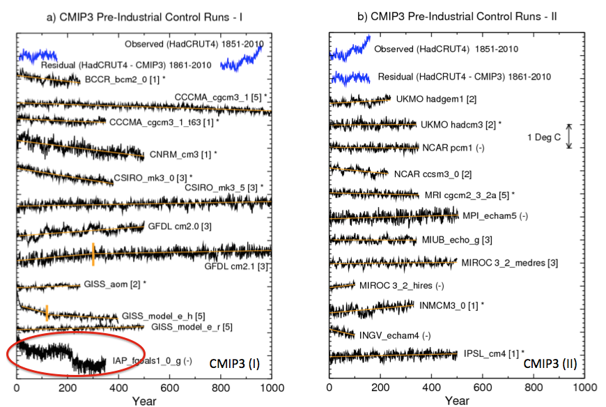
From Knutson et al 2013
Figure 1
Perhaps this is correct. Or perhaps the jump in simulated temperature is the climate model capturing natural climate variability.
The authors do comment:
As noted by Wittenberg (2009) and Vecchi and Wittenberg (2010), long-running control runs suggest that internally generated SST variability, at least in the ENSO region, can vary substantially between different 100-yr periods (approximately the length of record used here for observations), which again emphasizes the caution that must be placed on comparisons of modeled vs. observed internal variability based on records of relatively limited duration.
The first paper referenced, Wittenberg 2009, was the paper we looked at in Part Six – El Nino.
So is the “caution” that comes from that study included in the probability of our models ability to simulate natural variability?
In reality, questions about internal variability are not really discussed. Trends are removed, models with discontinuities are artifacts. What is left? This paper essentially takes the modeling output from the CMIP3 and CMIP5 archives (with and without GHG forcing) as a given and applies some tests.
Ribes & Terray 2013
This was a “Part II” paper and they said:
We use the same estimates of internal variability as in Ribes et al. 2013 [the “Part I”].
These are based on intra-ensemble variability from the above CMIP5 experiments as well as pre-industrial simulations from both the CMIP3 and CMIP5 archives, leading to a much larger sample than previously used (see Ribes et al. 2013 for details about ensembles). We then implicitly assume that the multi-model internal variability estimate is reliable.
[Emphasis added]. The Part I paper said:
An estimate of internal climate variability is required in detection and attribution analysis, for both optimal estimation of the scaling factors and uncertainty analysis.
Estimates of internal variability are usually based on climate simulations, which may be control simulations (i.e. in the present case, simulations with no variations in external forcings), or ensembles of simulations with the same prescribed external forcings.
In the latter case, m – 1 independent realisations of pure internal variability may be obtained by subtracting the ensemble mean from each member (assuming again additivity of the responses) and rescaling the result by a factor √(m/(m-1)) , where m denotes the number of members in the ensemble.
Note that estimation of internal variability usually means estimation of the covariance matrix of a spatio-temporal climate-vector, the dimension of this matrix potentially being high. We choose to use a multi-model estimate of internal climate variability, derived from a large ensemble of climate models and simulations. This multi-model estimate is subject to lower sampling variability and better represents the effects of model uncertainty on the estimate of internal variability than individual model estimates. We then simultaneously consider control simulations from the CMIP3 and CMIP5 archives, and ensembles of historical simulations (including simulations with individual sets of forcings) from the CMIP5 archive.
All control simulations longer than 220 years (i.e. twice the length of our study period) and all ensembles (at least 2 members) are used. The overall drift of control simulations is removed by subtracting a linear trend over the full period.. We then implicitly assume that this multi- model internal variability estimate is reliable.
[Emphasis added]. So two approaches to evaluate internal variability – one approach uses GCM runs with no GHG forcing; and the other approach uses the variation between different runs of the same model (with GHG forcing) to estimate natural variability. Drift is removed as “an error”.
Chapter 10 on Spatial Trends
The IPCC report also reviews the spatial simulations compared with spatial observations, p. 880:
Figure 10.2a shows the pattern of annual mean surface temperature trends observed over the period 1901–2010, based on Hadley Centre/ Climatic Research Unit gridded surface temperature data set 4 (Had- CRUT4). Warming has been observed at almost all locations with sufficient observations available since 1901.
Rates of warming are generally higher over land areas compared to oceans, as is also apparent over the 1951–2010 period (Figure 10.2c), which simulations indicate is due mainly to differences in local feedbacks and a net anomalous heat transport from oceans to land under GHG forcing, rather than differences in thermal inertia (e.g., Boer, 2011). Figure 10.2e demonstrates that a similar pattern of warming is simulated in the CMIP5 simulations with natural and anthropogenic forcing over the 1901–2010 period. Over most regions, observed trends fall between the 5th and 95th percentiles of simulated trends, and van Oldenborgh et al. (2013) find that over the 1950–2011 period the pattern of observed grid cell trends agrees with CMIP5 simulated trends to within a combination of model spread and internal variability..
van Oldenborgh et al (2013)
Let’s take a look at van Oldenborgh et al (2013).
There’s a nice video of (I assume) the lead author talking about the paper and comparing the probabilistic approach used in weather forecasts with that of climate models (see Ensemble Forecasting). I recommend the video for a good introduction to the topic of ensemble forecasting.
With weather forecasting the probability comes from running ensembles of weather models and seeing, for example, how many simulations predict rain vs how many do not. The proportion is the probability of rain. With weather forecasting we can continually review how well the probabilities given by ensembles match the reality. Over time we will build up a set of statistics of “probability of rain” and compare with the frequency of actual rainfall. It’s pretty easy to see if the models are over-confident or under-confident.
Here is what the authors say about the problem and how they approached it:
The ensemble is considered to be an estimate of the probability density function (PDF) of a climate forecast. This is the method used in weather and seasonal forecasting (Palmer et al 2008). Just like in these fields it is vital to verify that the resulting forecasts are reliable in the definition that the forecast probability should be equal to the observed probability (Joliffe and Stephenson 2011).
If outcomes in the tail of the PDF occur more (less) frequently than forecast the system is overconfident (underconfident): the ensemble spread is not large enough (too large).
In contrast to weather and seasonal forecasts, there is no set of hindcasts to ascertain the reliability of past climate trends per region. We therefore perform the verification study spatially, comparing the forecast and observed trends over the Earth. Climate change is now so strong that the effects can be observed locally in many regions of the world, making a verification study on the trends feasible. Spatial reliability does not imply temporal reliability, but unreliability does imply that at least in some areas the forecasts are unreliable in time as well. In the remainder of this letter we use the word ‘reliability’ to indicate spatial reliability.
[Emphasis added]. The paper first shows the result for one location, the Netherlands, with the spread of model results vs the actual result from 1950-2011:
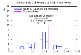
from van Oldenborgh et al 2013
Figure 2
We can see that the models are overall mostly below the observation. But this is one data point. So if we compared all of the datapoints – and this is on a grid of 2.5º – how do the model spreads compare with the results? Are observations above 95% of the model results only 5% of the time? Or more than 5% of the time? And are observations below 5% of the model results only 5% of the time?
We can see that the frequency of observations in the bottom 5% of model results is about 13% and the frequency of observations in the top 5% of model results is about 20%. Therefore the models are “overconfident” in spatial representation of the last 60 year trends:
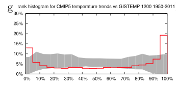
From van Oldenborgh et al 2013
Figure 3
We investigated the reliability of trends in the CMIP5 multi-model ensemble prepared for the IPCC AR5. In agreement with earlier studies using the older CMIP3 ensemble, the temperature trends are found to be locally reliable. However, this is due to the differing global mean climate response rather than a correct representation of the spatial variability of the climate change signal up to now: when normalized by the global mean temperature the ensemble is overconfident. This agrees with results of Sakaguchi et al (2012) that the spatial variability in the pattern of warming is too small. The precipitation trends are also overconfident. There are large areas where trends in both observational dataset are (almost) outside the CMIP5 ensemble, leading us to conclude that this is unlikely due to faulty observations.
It’s probably important to note that the author comments in the video “on the larger scale the models are not doing so badly”.
It’s an interesting paper. I’m not clear whether the brief note in AR5 reflects the paper’s conclusions.
Jones et al 2013
It was reassuring to finally find a statement that confirmed what seemed obvious from the “omissions”:
A basic assumption of the optimal detection analysis is that the estimate of internal variability used is comparable with the real world’s internal variability.
Surely I can’t be the only one reading Chapter 10 and trying to understand the assumptions built into the “with 95% confidence” result. If Chapter 10 is only aimed at climate scientists who work in the field of attribution and detection it is probably fine not to actually mention this minor detail in the tight constraints of only 60 pages.
But if Chapter 10 is aimed at a wider audience it seems a little remiss not to bring it up in the chapter itself.
I probably missed the stated caveat in chapter 10’s executive summary or introduction.
The authors continue:
As the observations are influenced by external forcing, and we do not have a non-externally forced alternative reality to use to test this assumption, an alternative common method is to compare the power spectral density (PSD) of the observations with the model simulations that include external forcings.
We have already seen that overall the CMIP5 and CMIP3 model variability compares favorably across different periodicities with HadCRUT4-observed variability (Figure 5). Figure S11 (in the supporting information) includes the PSDs for each of the eight models (BCC-CSM1-1, CNRM-CM5, CSIRO- Mk3-6-0, CanESM2, GISS-E2-H, GISS-E2-R, HadGEM2- ES and NorESM1-M) that can be examined in the detection analysis.
Variability for the historical experiment in most of the models compares favorably with HadCRUT4 over the range of periodicities, except for HadGEM2-ES whose very long period variability is lower due to the lower overall trend than observed and for CanESM2 and bcc-cm1-1 whose decadal and higher period variability are larger than observed.
While not a strict test, Figure S11 suggests that the models have an adequate representation of internal variability—at least on the global mean level. In addition, we use the residual test from the regression to test whether there are any gross failings in the models representation of internal variability.
Figure S11 is in the supplementary section of the paper:
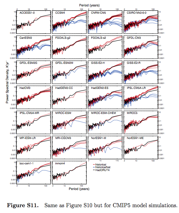
From Jones et al 2013, figure S11
Figure 4
From what I can see, this demonstrates that the spectrum of the models’ internal variability (“historicalNat”) is different from the spectrum of the models’ forced response with GHG changes (“historical”).
It feels like my quantum mechanics classes all over again. I’m probably missing something obvious, and hopefully knowledgeable readers can explain.
Chapter 9 of AR5 – Climate Models’ Representation of Internal Variability
Chapter 9, reviewing models, stretches to over 80 pages. The section on internal variability is section 9.5.1:
However, the ability to simulate climate variability, both unforced internal variability and forced variability (e.g., diurnal and seasonal cycles) is also important. This has implications for the signal-to-noise estimates inherent in climate change detection and attribution studies where low-frequency climate variability must be estimated, at least in part, from long control integrations of climate models (Section 10.2).
Section 9.5.3:
In addition to the annual, intra-seasonal and diurnal cycles described above, a number of other modes of variability arise on multi-annual to multi-decadal time scales (see also Box 2.5). Most of these modes have a particular regional manifestation whose amplitude can be larger than that of human-induced climate change. The observational record is usually too short to fully evaluate the representation of variability in models and this motivates the use of reanalysis or proxies, even though these have their own limitations.
Figure 9.33a shows simulated internal variability of mean surface temperature from CMIP5 pre-industrial control simulations. Model spread is largest in the tropics and mid to high latitudes (Jones et al., 2012), where variability is also large; however, compared to CMIP3, the spread is smaller in the tropics owing to improved representation of ENSO variability (Jones et al., 2012). The power spectral density of global mean temperature variance in the historical simulations is shown in Figure 9.33b and is generally consistent with the observational estimates. At longer time scale of the spectra estimated from last millennium simulations, performed with a subset of the CMIP5 models, can be assessed by comparison with different NH temperature proxy records (Figure 9.33c; see Chapter 5 for details). The CMIP5 millennium simulations include natural and anthropogenic forcings (solar, volcanic, GHGs, land use) (Schmidt et al., 2012).
Significant differences between unforced and forced simulations are seen for time scale larger than 50 years, indicating the importance of forced variability at these time scales (Fernandez-Donado et al., 2013). It should be noted that a few models exhibit slow background climate drift which increases the spread in variance estimates at multi-century time scales.
Nevertheless, the lines of evidence above suggest with high confidence that models reproduce global and NH temperature variability on a wide range of time scales.
[Emphasis added]. Here is fig 9.33:
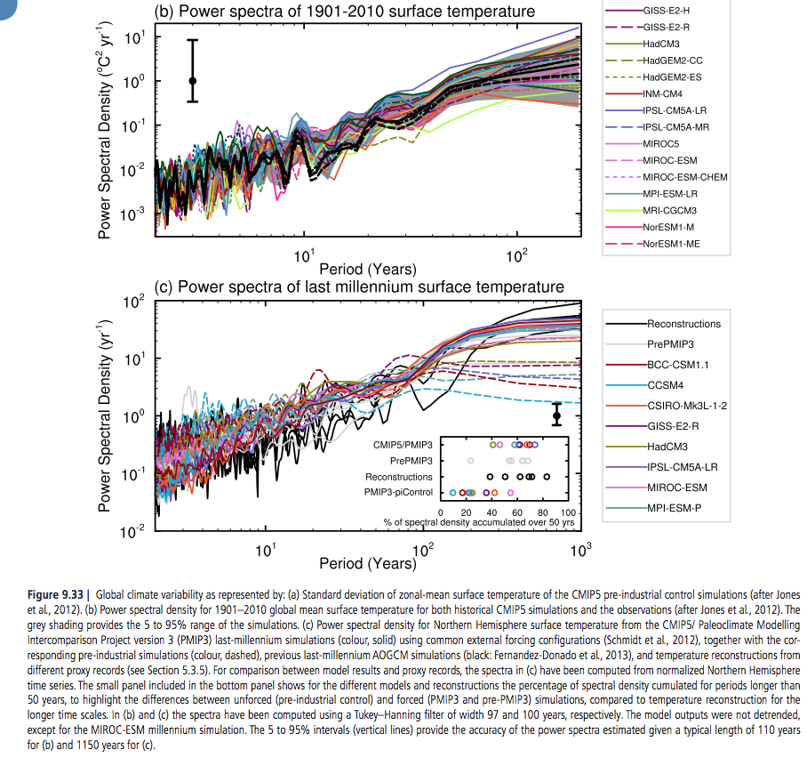
From IPCC AR5 Chapter 10
Figure 5 – Click to Expand
The bottom graph shows the spectra of the last 1,000 years – black line is observations (reconstructed from proxies), dashed lines are without GHG forcings, and solid lines are with GHG forcings.
In later articles we will review this in more detail.
Conclusion
The IPCC report on attribution is very interesting. Most attribution studies compare observations of the last 100 – 150 years with model simulations using anthropogenic GHG changes and model simulations without (note 3).
The results show a much better match for the case of the anthropogenic forcing.
The primary method is with global mean surface temperature, with more recent studies also comparing the spatial breakdown. We saw one such comparison with van Oldenborgh et al (2013). Jones et al (2013) also reviews spatial matching, finding a better fit (of models & observations) for the last half of the 20th century than the first half. (As with van Oldenborgh’s paper, the % match outside 90% of model results was greater than 10%).
My question as I first read Chapter 10 was how was the high confidence attained and what is a fingerprint?
I was led back, by following the chain of references, to one of the early papers on the topic (1996) that also had similar high confidence. (We saw this in Part Three). It was intriguing that such confidence could be attained with just a few “no forcing” model runs as comparison, all of which needed “flux adjustment”. Current models need much less, or often zero, flux adjustment.
In later papers reviewed in AR5, “no forcing” model simulations that show temperature trends or jumps are often removed or adjusted.
I’m not trying to suggest that “no forcing” GCM simulations of the last 150 years have anything like the temperature changes we have observed. They don’t.
But I was trying to understand what assumptions and premises were involved in attribution. Chapter 10 of AR5 has been valuable in suggesting references to read, but poor at laying out the assumptions and premises of attribution studies.
For clarity, as I stated in Part Three:
..as regular readers know I am fully convinced that the increases in CO2, CH4 and other GHGs over the past 100 years or more can be very well quantified into “radiative forcing” and am 100% in agreement with the IPCCs summary of the work of atmospheric physics over the last 50 years on this topic. That is, the increases in GHGs have led to something like a “radiative forcing” of 2.8 W/m²..
..Therefore, it’s “very likely” that the increases in GHGs over the last 100 years have contributed significantly to the temperature changes that we have seen.
So what’s my point?
Chapter 10 of the IPCC report fails to highlight the important assumptions in the attribution studies. Chapter 9 of the IPCC report has a section on centennial/millennial natural variability with a “high confidence” conclusion that comes with little evidence and appears to be based on a cursory comparison of the spectral results of the last 1,000 years proxy results with the CMIP5 modeling studies.
In chapter 10, the executive summary states:
..given that observed warming since 1951 is very large compared to climate model estimates of internal variability (Section 10.3.1.1.2), which are assessed to be adequate at global scale (Section 9.5.3.1), we conclude that it is virtually certain [99-100%] that internal variability alone cannot account for the observed global warming since 1951.
[Emphasis added]. I agree, and I don’t think anyone who understands radiative forcing and climate basics would disagree. To claim otherwise would be as ridiculous as, for example, claiming that tiny changes in solar insolation from eccentricity modifications over 100 kyrs cause the end of ice ages, whereas large temperature changes during these ice ages have no effect (see note 2).
The executive summary also says:
It is extremely likely [95–100%] that human activities caused more than half of the observed increase in GMST from 1951 to 2010.
The idea is plausible, but the confidence level is dependent on a premise that is claimed via one graph (fig 9.33) of the spectrum of the last 1,000 years. High confidence (“that models reproduce global and NH temperature variability on a wide range of time scales”) is just an opinion.
It’s crystal clear, by inspection of CMIP3 and CMIP5 model results, that models with anthropogenic forcing match the last 150 years of temperature changes much better than models held at constant pre-industrial forcing.
I believe natural variability is a difficult subject which needs a lot more than a cursory graph of the spectrum of the last 1,000 years to even achieve low confidence in our understanding.
Chapters 9 & 10 of AR5 haven’t investigated “natural variability” at all. For interest, some skeptic opinions are given in note 4.
I propose an alternative summary for Chapter 10 of AR5:
It is extremely likely [95–100%] that human activities caused more than half of the observed increase in GMST from 1951 to 2010, but this assessment is subject to considerable uncertainties.
Articles in the Series
Natural Variability and Chaos – One – Introduction
Natural Variability and Chaos – Two – Lorenz 1963
Natural Variability and Chaos – Three – Attribution & Fingerprints
Natural Variability and Chaos – Four – The Thirty Year Myth
Natural Variability and Chaos – Five – Why Should Observations match Models?
Natural Variability and Chaos – Six – El Nino
Natural Variability and Chaos – Seven – Attribution & Fingerprints Or Shadows?
Natural Variability and Chaos – Eight – Abrupt Change
References
Multi-model assessment of regional surface temperature trends, TR Knutson, F Zeng & AT Wittenberg, Journal of Climate (2013) – free paper
Attribution of observed historical near surface temperature variations to anthropogenic and natural causes using CMIP5 simulations, Gareth S Jones, Peter A Stott & Nikolaos Christidis, Journal of Geophysical Research Atmospheres (2013) – paywall paper
Application of regularised optimal fingerprinting to attribution. Part II: application to global near-surface temperature, Aurélien Ribes & Laurent Terray, Climate Dynamics (2013) – free paper
Application of regularised optimal fingerprinting to attribution. Part I: method, properties and idealised analysis, Aurélien Ribes, Serge Planton & Laurent Terray, Climate Dynamics (2013) – free paper
Reliability of regional climate model trends, GJ van Oldenborgh, FJ Doblas Reyes, SS Drijfhout & E Hawkins, Environmental Research Letters (2013) – free paper
Notes
Note 1: CMIP = Coupled Model Intercomparison Project. CMIP3 was for AR4 and CMIP5 was for AR5.
At a September 2008 meeting involving 20 climate modeling groups from around the world, the WCRP’s Working Group on Coupled Modelling (WGCM), with input from the IGBP AIMES project, agreed to promote a new set of coordinated climate model experiments. These experiments comprise the fifth phase of the Coupled Model Intercomparison Project (CMIP5). CMIP5 will notably provide a multi-model context for
1) assessing the mechanisms responsible for model differences in poorly understood feedbacks associated with the carbon cycle and with clouds
2) examining climate “predictability” and exploring the ability of models to predict climate on decadal time scales, and, more generally
3) determining why similarly forced models produce a range of responses…
From the website link above you can read more. CMIP5 is a substantial undertaking, with massive output of data from the latest climate models. Anyone can access this data, similar to CMIP3. Here is the Getting Started page.
And CMIP3:
In response to a proposed activity of the World Climate Research Programme (WCRP) Working Group on Coupled Modelling (WGCM), PCMDI volunteered to collect model output contributed by leading modeling centers around the world. Climate model output from simulations of the past, present and future climate was collected by PCMDI mostly during the years 2005 and 2006, and this archived data constitutes phase 3 of the Coupled Model Intercomparison Project (CMIP3). In part, the WGCM organized this activity to enable those outside the major modeling centers to perform research of relevance to climate scientists preparing the Fourth Asssessment Report (AR4) of the Intergovernmental Panel on Climate Change (IPCC). The IPCC was established by the World Meteorological Organization and the United Nations Environmental Program to assess scientific information on climate change. The IPCC publishes reports that summarize the state of the science.
This unprecedented collection of recent model output is officially known as the “WCRP CMIP3 multi-model dataset.” It is meant to serve IPCC’s Working Group 1, which focuses on the physical climate system — atmosphere, land surface, ocean and sea ice — and the choice of variables archived at the PCMDI reflects this focus. A more comprehensive set of output for a given model may be available from the modeling center that produced it.
With the consent of participating climate modelling groups, the WGCM has declared the CMIP3 multi-model dataset open and free for non-commercial purposes. After registering and agreeing to the “terms of use,” anyone can now obtain model output via the ESG data portal, ftp, or the OPeNDAP server.
As of July 2009, over 36 terabytes of data were in the archive and over 536 terabytes of data had been downloaded among the more than 2500 registered users
Note 2: This idea is explained in Ghosts of Climates Past -Eighteen – “Probably Nonlinearity” of Unknown Origin – what is believed and what is put forward as evidence for the theory that ice age terminations were caused by orbital changes, see especially the section under the heading: Why Theory B is Unsupportable.
Note 3: Some studies use just fixed pre-industrial values, and others compare “natural forcings” with “no forcings”.
“Natural forcings” = radiative changes due to solar insolation variations (which are not known with much confidence) and aerosols from volcanos. “No forcings” is simply fixed pre-industrial values.
Note 4: Chapter 11 (of AR5), p.982:
For the remaining projections in this chapter the spread among the CMIP5 models is used as a simple, but crude, measure of uncertainty. The extent of agreement between the CMIP5 projections provides rough guidance about the likelihood of a particular outcome. But—as partly illustrated by the discussion above—it must be kept firmly in mind that the real world could fall outside of the range spanned by these particular models. See Section 11.3.6 for further discussion.
And p. 1004:
It is possible that the real world might follow a path outside (above or below) the range projected by the CMIP5 models. Such an eventuality could arise if there are processes operating in the real world that are missing from, or inadequately represented in, the models. Two main possibilities must be considered: (1) Future radiative and other forcings may diverge from the RCP4.5 scenario and, more generally, could fall outside the range of all the RCP scenarios; (2) The response of the real climate system to radiative and other forcing may differ from that projected by the CMIP5 models. A third possibility is that internal fluctuations in the real climate system are inadequately simulated in the models. The fidelity of the CMIP5 models in simulating internal climate variability is discussed in Chapter 9..
..The response of the climate system to radiative and other forcing is influenced by a very wide range of processes, not all of which are adequately simulated in the CMIP5 models (Chapter 9). Of particular concern for projections are mechanisms that could lead to major ‘surprises’ such as an abrupt or rapid change that affects global-to-continental scale climate.
Several such mechanisms are discussed in this assessment report; these include: rapid changes in the Arctic (Section 11.3.4 and Chapter 12), rapid changes in the ocean’s overturning circulation (Chapter 12), rapid change of ice sheets (Chapter 13) and rapid changes in regional monsoon systems and hydrological climate (Chapter 14). Additional mechanisms may also exist as synthesized in Chapter 12. These mechanisms have the potential to influence climate in the near term as well as in the long term, albeit the likelihood of substantial impacts increases with global warming and is generally lower for the near term.
And p. 1009 (note that we looked at Rowlands et al 2012 in Part Five – Why Should Observations match Models?):
The CMIP3 and CMIP5 projections are ensembles of opportunity, and it is explicitly recognized that there are sources of uncertainty not simulated by the models. Evidence of this can be seen by comparing the Rowlands et al. (2012) projections for the A1B scenario, which were obtained using a very large ensemble in which the physics parameterizations were perturbed in a single climate model, with the corresponding raw multi-model CMIP3 projections. The former exhibit a substantially larger likely range than the latter. A pragmatic approach to addressing this issue, which was used in the AR4 and is also used in Chapter 12, is to consider the 5 to 95% CMIP3/5 range as a ‘likely’ rather than ‘very likely’ range.
Replacing ‘very likely’ = 90–100% with ‘likely 66–100%’ is a good start. How does this recast chapter 10?
And Chapter 1 of AR5, p. 138:
Model spread is often used as a measure of climate response uncertainty, but such a measure is crude as it takes no account of factors such as model quality (Chapter 9) or model independence (e.g., Masson and Knutti, 2011; Pennell and Reichler, 2011), and not all variables of interest are adequately simulated by global climate models..
..Climate varies naturally on nearly all time and space scales, and quantifying precisely the nature of this variability is challenging, and is characterized by considerable uncertainty.
[Emphasis added in all bold sections above]


I wasn’t sure whether to put this comment here or in the previous article on El Nino. There’s no right answer.
This is from A Pacific Centennial Oscillation Predicted by Coupled GCMs, Karnauskas, Smerdon, Seager & Gonzalez-Rouco, Journal of Climate (2012):
– As a side note, from where this (one of 50) open tabs was sitting on my Mac, it probably came from a comment, so thanks to whoever cited this paper.
OK, let’s throw down a gauntlet for the sake of argument.
Before starting the argument, the explanation for the observed (late) 20th century warming as proposed by IPCC I consider physically plausible and there is no doubt I my mind that what is described in IPCC could be what has been and is happening in reality. But that does not necessarily make it true.
So, let’s start with the paper below, which discusses a case of ‘spontaneous’ decadal/centennial unforced (and sort of unexpected) variability in the global earth-system model EC-EARTH.
…
Drijfhout, Sybren, Gleeson, Emily, Dijkstra, Henk A. and Livina, Valerie (2013) Spontaneous abrupt climate change due to an atmospheric blocking–sea-ice–ocean feedback in an unforced climate model simulation. Proceedings of the National Academy of Sciences, 110, (49), 19713 -19718. (doi:10.1073/pnas.1304912110).
“Abstract. There is a long-standing debate about whether climate models are able to simulate large, abrupt events that characterized past climates. Here, we document a large, spontaneously occurring cold event in a preindustrial control run of a new climate model. The event is comparable to the Little Ice Age both in amplitude and duration; it is abrupt in its onset and termination, and it is characterized by a long period in which the atmospheric circulation over the North Atlantic is locked into a state with enhanced blocking. To simulate this type of abrupt climate change, climate models should possess sufficient resolution to correctly represent atmospheric blocking and a sufficiently sensitive sea-ice model.”
From the conclusions:
“The lesson learned from this study is that the climate system is capable of generating large, abrupt climate excursions without externally imposed perturbations. Also, because such episodic events occur spontaneously, they may have limited predictability.”
The whole paper is well worth a read, but I’ll leave that to the interested reader.
…
So, the virtual climate world is advancing to a level where spontaneous decadal/centennial variability is possible (i.e. not caused by drifts or other unphysical processes).
There are many interesting aspects, question and possible consequences with regard this paper, which I will not touch upon here.
Instead, let’s focus on what this means for the attribution question, which is not touched upon by the authors.
1) How do we know that for example the Little Ice Age (LIA) has not been a manifestation of the same type of variability (actually the paper implies it may very well be)?
2) If this spontaneous type of variability is possible in the climate system, how do we then know that the current warming is not the result of a rebound from the LIA, and if so, how large is that rebound (i.e. most 20th century warming, part of it, hardly any of it?)?
3) Can climate models that are unable to simulate this type of spontaneous climate variability be used for attribution, as the attribution studies have always assumed that this type of variability does not occur in reality?
4) What does that mean for attribution in past studies (incl. IPCC) where climate model drift and climate model anomalies have been ascribed to unphysical processes.
With regard to (2) it could be argued that the LIA is the ‘odd one out’, i.e. the LIA is an unusual and rather unique period during the Holocene (see GISP Greenland ice core).
Logically, as most climate models have not yet been shown to be able to generate spontaneous natural warming, there is no possibility to quantify how much warming needs to be explained. Furthermore, the answer to (3) then could be a clear ‘no’, and a possible answer to (4) is that the methodology used in past attribution studies as well as the results from those studies should be reassessed, thus judging past (IPCC) attribution results as not being useful.
In summary, the basic question is this: do we have sufficient understanding of decadal to centennial scale climate variability to argue that 20th century warming cannot be explained by ‘internal variability’, as concluded per IPCC?
I would argue that results from this paper question that idea.
Cheers, Jos.
(ps. yes, the man in the video is indeed GJ van Oldenborgh).
Nice to see that people are sharing the same questions. Thanks for your comment.
Jos,
Thanks for citing this paper, it is very interesting on a number of levels. I will probably use it in a forthcoming article.
Thank you for your presentation of the thoughts behind model development and how to verify. I have some questions about how to understand natural climate variations. There have been some discussions on recovery or rebound from Little Ice Age. If it is right that the world cooled down over some hundred years, that the ocean cooled, that ocean stratification became stronger, that the termocline depth moved, that the sst at polar regions became a couple of degrees colder, would it not be a thermal imbalance that had to be balanced? Could that be a natural cause of the earth energy uptake and warming? When an object is cooled down, it should take up energy to come into balance. This culd be the primary natural cause of the last 250 years of climate change. I wonder how this is represented in climate models. And I am not arguing against anthropogenetic driven forcings. It must be a big task to find out: How much of the one, how much of the other.
How much of the one (natural), how much of the other (anthropogenetic). I think some models give an answer, as when the model GM2,1 (previous SOD post) calculate a climate sensitivity of 3,4 degrees
I’m not quite sure what is meant by “rebound”.
Heat content (as evidenced by temperature) does not behave like a bouncing ball. If you put a room-temperature fork in a freezer, it will begin to cool. This occurs because the fork, being warmer than the remainder of the freezer’s contents, releases more energy than it absorbs. The other contents, being colder than the fork, absorb more energy than they release, thus becoming slightly warmer. The end result of this continuous energy exchange is that the fork and the other contents eventually attain the same temperature, at which they will remain forever until something changes (e.g., you open the door, the freezer turns on, heat leaks through the freezer’s insulation, etc).
if borehole temperatures lag athmospheric temperatures with a couple of centuries, It take time to assimilate energy. it will make a small bouncing. Perhaps OHC is operating in a similar way, with far more energies.
The rate of energy transfer does indeed vary greatly, depending upon the circumstances (e.g., conduction in rock vs. convection and radiation in air). I don’t understand, though, how this relates to some concept of “rebound”.
I think it’s just a language issue – we’re dealing with a dynamic system. If an impulse caused the LIA when it ceased the temperature would rebound (and depending on how complex the atmosphere is one may get overshoots).
So using your analogy if you stick your fork in the fridge it drops down in temp, and when you take it out it rebounds.
What is meant by “impulse”? Do you mean that if the LIA was caused by a dip in solar activity, say from S to 0.99S, that when solar activity returned to S global average temperature would return to its pre-LIA value? I don’t have a problem with that formulation (though it’s conceivable that the climate might enter some different state). I do, however, reject the idea that temperature changes have some sort of momentum (e.g., that a room-temperature fork stuck in a flame will continue to warm for awhile after it’s removed from the flame), as it violates conservation of energy.
Perhaps have a glance at the kinetic theory of temperatures.
And I will learn something about “rebounds” and “impulses” that contravenes conservation of energy? I’d like to understand what is meant by the oft-cited “rebound from the LIA” as an explanation for post-Industrial Revolution warming. Do you have an explanation that’s not unphysical?
I was in a hurry before, but did you have a look? It struck me you were misunderstanding “momentum” in this context and it was getting in the way of you picking up the quite simple use of the term “rebound”.
Using that theory you will see that the temp is just a measure of the kinetic energy of the molecules, and yes in this sense temp has momentum – its what makes the temp stay the same unless someone does some work on it – speeding up the molecules (aka heating) or slowing them down (aka cooling).
And continuing the analogy just as to get a bounce on a ball you need another object to turn the ball around, so atmosphere at the surface needed something to interact with to “bounce” it out of the LIA. It could of course have been something else in the oceans, the land, the atmosphere or extraterrestrial.
So the expression “rebound from the LIA” has no meaning as an explanation for post-Industrial Revolution warming, since it merely speculates that something changed to cause temperatures to rise.
Correct.
However it potentially carries with it the idea that the transition to the LIA stored up energy elsewhere in the system (think ball attached to a rubber band – the energy ends up in the rubber band) that then got transferred back to the surface atmosphere to fuel the rebound (the rubber band gives it up).
The question being discussed here is whether that kind of sloshing of energy around in the the oceans, the land and the atmosphere might be within the bounds of normal behaviour of the earth, or whether we need ET.
Actually that analogy isn’t quite correct. The other option being discussed is whether one of the processes in the atmosphere – the actions of humans on the earth – is changing the “natural order” to predispose a particular response.
I don’t believe enough energy could be stored in the system (to me it would have to be oceans) in a way that would allow it to come back and sustain a natural rebound of the GMT from the LIA.
JCH,
You’re thinking in static terms. It’s not about the heat content so much as the heat flow. For example, if more heat flows into the deep ocean, the surface will cool. In the converse, the surface will warm. There’s always heat flowing into the system from the sun and radiating out to space. Energy does not have to come back from the ocean for the surface to warm.
There’s also the distribution. You can have a lower global average temperature with the same radiation to space if the Tropics warm and the higher latitudes cool. Changing ocean currents could do that. The extreme situation is for a non-rotating sphere. The average temperature of the sphere will be a lot lower than for a rapidly rotating sphere. Yet the same amount of power will be absorbed and radiated back to space. See also Earth’s moon.
Dewitt – but he referred to stored energy coming back. Saying the surface can be warmed, or cooled, in a variety of other ways doesn’t address the issue. Can stored energy, energy safety put away in place that does not show up in the very low GMT of the LIA, cause a GMT rebound from the LIA? I do not believe it can. I agree that there are other natural means of raising the temperature of the surface from LIA levels, but I’m dubious these other means, of their own accord, could cause a rebound to MWP levels.
JCH,
The question at the top of the thread from nobodyknows was about energy imbalance:
He did not refer to energy coming back. Nor, in fact, did HAS:
One can, of course, misread anything, thereby creating a straw man argument, rebutting something that was not, in fact, the original proposition.
JCH you should include the oceans as part of the system under consideration and you should also consider all the ways energy can be stored – it isn’t just thermal or kinetic (gases moving around). Phase changes and chemical reactions can lock up or release energy.
Also temp changes and other related changes can actually change the way the system works. We see that with our analogy – if you put the ball in liquid nitrogen before throwing it at the wall the energy goes into breaking the ball up rather than bouncing it back. As I noted this is what increasing concentrations of GHG are doing – but equally there might be countervailing influences.
You are also concerned about not being able to “see” the store. Apart from drawing attention to the various ways it might be stored it is quite possible that we are seeing artifacts of processes that are operating on time scales we can’t resolve in time (for example).
nobodyknows,
Thinking about climate like this – like energy balance models – is a great starting point.
But – the hypothesis that climate is actually like this, some kind of linear response model, is very hard to demonstrate and no one tries to do it, only at best arguing for the benefits that come from applying simple models to the climate system (see my comment below).
A nice study of control systems with negative feedback is the simple idea – you get to apply a change and the system drives the output back to where it was before, or to where it was plus the change x the feedback.
Then try a control system with positive feedback – it gets much more complicated.
The climate system has lots of feedbacks, both positive and negative, and there is no evidence in favor of the idea that they are constant or linear.
A brief follow up.
SoD, I don’t know if you are aware of the works of Irish meteorologist Prof. J.R. Bates, but he has also been exploring the concept of climate sensitivity and in particular what happens if you add a bit of complexity to the concept.
In essence, one of the things he argues is that if you accept that the climate system consists of more than one sub-system that interact, like tropics and extra-tropics, counter-intuitive things can start to happen. And distinguishing between tropics and extra-tropics is not completely stupid, there are some fundamental differences between the two.
The abstract of a 2010 paper notes:
Abstract. A theoretical investigation of climate stability and sensitivity is carried out using three simple linearized models based on the top-of-the-atmosphere energy budget. The simplest is the zero-dimensional model (ZDM) commonly used as a conceptual basis for climate sensitivity and feedback studies. The others are two-zone models with tropics and extratropics of equal area; in the first of these (Model A), the dynamical heat transport (DHT) between the zones is implicit, in the second (Model B) it is explicitly parameterized. It is found that the stability and sensitivity properties of the ZDM and Model A are very similar, both depending only on the global-mean radiative response coefficient and the global-mean forcing. The corresponding properties of Model B are more complex, depending asymmetrically on the separate tropical and extratropical values of these quantities, as well as on the DHT coefficient. Adopting Model B as a benchmark, conditions are found under which the validity of the ZDM and Model A as climate sensitivity models holds. It is shown that parameter ranges of physical interest exist for which such validity may not hold. The 2 × CO2 sensitivities of the simple models are studied and compared. Possible implications of the results for sensitivities derived from GCMs and palaeoclimate data are suggested. Sensitivities for more general scenarios that include negative forcing in the tropics (due to aerosols, inadvertent or geoengineered) are also studied. Some unexpected outcomes are found in this case. THESE INCLUDE THE POSSIBILITY OF A NEGATIVE GLOBAL-MEAN TEMPERATURE RESPONSE TO A POSITIVE GLOBAL-MEAN FORCING, AND VICE VERSA. [emphasis added]
If that last remark doesn’t trigger your interest, I don’t know what would …
http://link.springer.com/article/10.1007%2Fs00382-010-0966-0
http://www.raybates.net/
Jos,
Interesting (paper by Bates). I had just started building a model like this (well a bit more complicated) to show what happens with a few regions and a few different feedbacks on a few timescales.
Since finding various papers (the El Nino paper by Wittenberg in 2009, the 2014 followup, the paper you highlighted by Drijfhout..) actually demonstrating with GCMs some of the points the model was going to demonstrate perhaps I am spared the work.
Thank you for your answer SOD, and for your clarification DeWitt Payne. After the last ice age it took 20000 years for the earth to recover, so that energy uptake and radiation out got into a kind of balance. I dont know how much energy uptake it was, but a huge amount. It was a sea level rise of about 120 m. The last 2000 years there has been a sea level change, up and down, of 30cm. This is also a huge amount of energy, and illustrate that it is a natural TOA imbalance. I think that the balance of radiation in and radiation out is only shortlived, even on timescales of some hundred years. An I have not seen a good explanation on the fluctuations of sea level.
The sea level rise and the ocean heat content rise gives a kind of storing of energy, like a kind of latent heat in the system, seen in the light of this fluctations.
Litterature: Sea level change in the Middle Ages and the Little Ice Age. F.J.P.M. Kwaad, physical geographer
The TOA imbalance needed for melting all the ice during deglaciation is not very large.
The rate of sea level rise was little more than 100 m in 100000 years, or 1 cm/year. That’s 10 kg/m^2. Melting 10 kg of ice takes 3.3 MJ. Dividing by the length of the year gives about 0.1 W/m^2, much less than the estimated present imbalance.
Correct.
However it potentially carries with it the idea that the transition to the LIA stored up energy elsewhere in the system (think ball attached to a rubber band – the energy ends up in the rubber band) that then got transferred back to the surface atmosphere to fuel the rebound (the rubber band gives it up). – HAS
I can’t imagine any place other than the oceans that could store enough energy to take the GMT at the depths of the LIA to the 2014 record GMT.
JCH,
I agree that the rubber band analogy is bad, at least for centennial to millennial scale fluctuations like the MWP to LIA to modern times. For glacial/interglacial transitions, though, some sort of non-linear with temperature storage and release seems likely.
In my defense the rubber band is just an analogy for anything that can convert energy from one form into another with an implication of reversibility to allow a bounce. This could be circulation patterns or even something ET supplies.
HAS,
The problem with energy conversion is the Second Law. You always get back less than you put in. And in the case of any mechanism that I can think of, it’s a lot less.
A change in the TOA energy balance through a change in cloud cover seems much more likely. If clouds are a negative feedback, than a fairly small increase in cloud cover will, over time, drop the average temperature quite a bit by decreasing input more than output decreases. If they’re a positive feedback, than a decrease will drop the temperature by decreasing output more than input.
Changes in cloud cover from changes in the magnitude and distribution of sea surface temperature has been postulated as the source of non-linearity in climate sensitivity with forcing over time, leading to much increased ECS over TCS. See comment and link to the paper here.
DeWitt, ta had missed that hadn’t been checking Lucia’s as regularly since the tempo dropped. I must say it doesn’t surprise me either.
As far as the rubber band thing is concerned perhaps regard it as the controller of the iris as it were 🙂
I think this is interesting in that earlier this year this was proposed as a cause of the pause, which seems plausible, and now as the cause of early 20th-century warming:
Early twentieth-century warming linked to tropical Pacific wind strength
UCAR-NCAR News
Minor correction:
IIRC, that’s because cloud cover is a fairly strong positive feedback in most GCM’s. It’s not at all clear that’s true in the real world.
Underlying problem here: the further back in time, the less our quantiative understanding of changes in climate. Temperature variability is less constrained further back: there is less and less information about spatial variations as well as about temporal changes. Let alone information about forcings and other climate variables like precipitation, wind, radiation, clouds, aerosols etc.). In particular the worse and worse temporal resolution is an issue: we want to know how climate varies one decadal to centennial time scales, but at some point the time resolution of climate proxies becomes insufficient to tell you much about variations on those time scales.
So, is it right that climate cooled down over some hundred years? Different reconstructions, different answers. Some say it did, some don’t. And was the cooling a global, hemispheric or regional issues? Again, different answers. And I’m not going there, as very unfriendly and nasty wars have been raging over that issue for years.
Which leaves a difficult puzzle to solve: if we have no clear grip on what climate looked like back then, how do we know what climate models should and shouldn’t do on timescales of decades and longer? The answer is that we don’t, and the review above of by SOD shows that papers and reports all struggle with this question. The most common approach has always been to simply assume that models are right on time scales of decades and longer, and that any drift or spontaneous changes were unphysical and could be ignored. But those are assumption that may not be justified, as suggested in my previous comment.
Various other approaches have been tried, but all come with their share of assumptions and issues, all the result of to the bottom line mentioned above: lack of sufficient information.
I’m afraid that won’t change very fast any time soon.
You’ll find similar thoughts in the works of Judith Curry on ClimEtc.
If unforced variability is larger than we are assuming, we must entertain not only the idea that it might constitute a positive percentage of the warming since 1880, but also the idea that it might constitute a *negative* percentage of that warming — i.e., that it might be cancelling some of the GHG-forced warming. Given these discussions so far, there is no reason to favor one idea over the other.
Meow,
This is correct.
This is just one of many studies that present natural variations in global change. I think many of them come to similar results. Theese studies maqke me favor some ideas over some other.
Using data to attribute episodes of warming and cooling in instrumental records
Ka-Kit Tung and Jiansong Zhou
Conclusion
Although there is a competing theory that the observed multidecadal
variability is forced by anthropogenic aerosols during the
industrial era (33), our present work showing that this variability
is quasi-periodic and extends at least 350 y into the past with
cycles in the preindustrial era argues in favor of it being naturally
recurrent and internally generated. This view is supported by
model results that relate the variability of the global-mean SST
to North Atlantic thermohaline circulation (30, 31, 35) and by
the existence of an AMO-like variability in control runs without
anthropogenic forcing (28). If this conclusion is correct, then the
following interpretation follows: The anthropogenic warming
started after the mid-19th century of Industrial Revolution. After
a slow start, the smoothed version of the warming trend has
stayed almost constant since 1910 at 0.07–0.08 °C/decade.
Superimposed on the secular trend is a natural multidecadal
oscillation of an average period of 70 y with significant amplitude
of 0.3–0.4 °C peak to peak, which can explain many historical
episodes of warming and cooling and accounts for 40% of the
observed warming since the mid-20th century and for 50% of the
previously attributed anthropogenic warming trend (55). Because
this large multidecadal variability is not random, but likely
recurrent based on its past behavior, it has predictive value. Not
taking the AMO into account in predictions of future warming
under various forcing scenarios may run the risk of overestimating
the warming for the next two to three decades, when
the AMO is likely in its down phase.
It is no coincidence that shifts in ocean and atmospheric indices occur at the same time as changes in the trajectory of global surface temperature. Our ‘interest is to understand – first the natural variability of climate – and then take it from there. So we were very excited when we realized a lot of changes in the past century from warmer to cooler and then back to warmer were all natural,’ Tsonis said.
In the 20th century – there were two multi-decadal warm periods and one cold. As well as presumably a warmer Sun – increasing in the first half of the century and staying high until at least 1985.
These multi-decadal periods involve chaotic shifts that are in principle deterministic but in practice incalculable. But it must be presumed that the change in temperature trajectory – at 1912, 1944, 1976 and 1998 – results from changes in cloud and water vapour or changes changes in energy partitioning between ocean and atmosphere. Or both.
Oceans are far too difficult and variable – and reliable observations far too short – to say much with any confidence. Clouds are only knowable in the satellite era. But what we do know is that – like the oceans – natural variability is huge.
‘Climate forcing results in an imbalance in the TOA radiation budget that has direct implications for global climate, but the large natural variability in the Earth’s radiation budget due to fluctuations in atmospheric and ocean dynamics complicates this picture.’ http://meteora.ucsd.edu/~jnorris/reprints/Loeb_et_al_ISSI_Surv_Geophys_2012.pdf
What do we know about cloud? Here’s a graph from Ben Laken and Enric Palle – which cross validates ISCCP-FD and MODIS using sea surface temperature in the tropical Pacific. The data says that the changes are very significant in recent warming – and in more recent non-warming.
Here’s a graph from AR4 – I haven’t graduated to AR5 yet.
I doubt very much that we understand carbon dioxide dynamics with any precision. Here’s a graph from Margret Steinthorsdottir et al 2013 – Stomatal proxy record of CO2 concentrations from the last termination suggests an important role for CO2 at climate change transitions – showing a very different dynamic to the ice cores.
So what do we know? Ocean and atmospheric circulation changes abruptly, the global energy dynamic changes dramatically and it seems associated with sea surface temparature in the Pacific and cloud formation.
Burgman et al (2008) used a variety of data sources to examine decadal variability of surface winds, water vapour (WV), outgoing longwave radiation (OLR) and clouds. They conclude that the ‘most recent climate shift, which occurred in the 1990s during a period of continuous satellite coverage, is characterized by a ‘La Niña’ SST pattern with significant signals in the central equatorial Pacific and also in the north-eastern subtropics. There is a clear westward shift in convection on the equator, and an apparent strengthening of the Walker circulation. In the north-eastern subtropics, SST cooling coinciding with atmospheric drying appears to be induced by changes in atmospheric circulation. There is no indication in the wind speed that the changes in SST or WV are a result of changes in the surface heat flux. There is also an increase in OLR which is consistent with the drying. Finally, there is evidence for an increase in cloud fraction in the stratus regions for the 1990s transition as seen in earlier studies.’
In a study that was widely interpreted as a demonstration of a positive global warming cloud feedback, Amy Clement and colleagues (2009) presented observational evidence of decadal change in cloud cover in surface observation of clouds from the Comprehensive Ocean Atmosphere Data Set (COADS). ‘Both COADS and adjusted ISCCP data sets show a shift toward more total cloud cover in the late 1990s, and the shift is dominated by low- level cloud cover in the adjusted ISCCP data. The longer COADS total cloud time series indicates that a similar magnitude shift toward reduced cloud cover occurred in the mid-1970s, and this earlier shift was also dominated by marine stratiform clouds. . . Our observational analysis indicates that increased SST and weaker subtropical highs will act to reduce NE Pacific cloud cover.’ As was clearly stated in the paper, the evidence was for a decadal cloud feedback negatively correlated with sea surface temperature in the region of the Pacific Decadal Oscillation. The feedbacks correspond exactly to changes in the Pacific multi-decadal pattern.
Much variability comes from changes in Pacific Ocean states – and we know without much doubt that El Nino frequency and intensity peaked in the 20th century in a 1000 year high.
Ellison asks
I am curious as to what kind of code word this is. No one uses the singular cloud in this context. This must be some sort of dog-whistle science.
The allusion was to this study.
http://scitation.aip.org/docserver/fulltext/aip/proceeding/aipcp/1531/10.1063/1.4804857/1.4804857.pdf?expires=1420142103&id=id&accname=guest&checksum=7D935937362218E54D97E2FF43DDF20E
Was I being too subtle? I am reading this at the moment.
‘A principle that unites every kind of complexity theorist,and they are a richly varied class (see §3 and §5, below), is that observable ‘reality’ pertaining to any field, physics, biology, chemistry, applied mathematics, economics, etc., is complex but this complexity emanates from simple building blocks – of concepts, methods and rules of interaction. Why, then, should this supreme scientist, of powerful intuitions, claim that nature is the realisation of the simplest conceivable mathematical ideas? Is it because even the ‘simplest conceivable mathematical ideas’, when realised in natural phenomena, become enveloped in complex manifestations and it is the task of the theorist to disentangle the apparent complexities and bare the hidden simplicities underpinned by, and in, simple laws and concepts? Such an interpretation would be welcomed by the complexity theorist who is in
the habit of showing how even unbelievably simple mechanisms are sufficient to demonstrate and encapsulate the complexity of phenomena in the natural, physical, biological, social and other phenomenological worlds.’
Click to access 7_03_vela.pdf
It has such a rare clarity and elegance – and is moreover sublimely topical – that comes with both an innate talent for language and with a soaring exposure to the finest expressions of the human mind. To quote Oscar Wilde – we are all in the gutter but some of us are looking at the cloud.
Nobody uses the singular “cloud” but apparently in some fiction that you quote. This is science and not fiction.
One of the largest contributions due to natural variability is that due to ENSO. This phenomena is perhaps more deterministic that scientists may presume. The fact that it is so closely linked to the Quasi-Biennial Oscillations (QBO), which have a strong periodicity along with some jitter, leads one to a possible deterministic analysis, such as I did here:
http://arxiv.org/abs/1411.0815
A group of us at the Azimuth Project are working on analyzing ENSO and El Nino to gain a better understanding of these quasi-periodic processes:
http://azimuth.mathforge.com
That is http://azimuth.mathforge.org not .com
‘El Nino southern oscillation (ENSO) behavior can be effectively modeled as a response to a 2nd-order Mathieu/Hill differential equation with periodic coefficients describing sloshing of a volume of water. The forcing of the equation derives from QBO, angular momentum changes synchronized with the Chandler wobble, and solar insolation variations. One regime change was identified in 1980.’
It was actually a joke – only on overcast nights do we look at cloud and not stars.
We have been through this before. You have an equation for standing waves on an elliptical surface modulated by other things that are more or less related to ENSO – but are no more predictable – and arbitrarily fitted to the SOI using a learning algorithm. The Sun may certainly be involved in ENSO and the length of day is almost certainly related to shifting wind speeds in the Pacific.
The QBO has obvious correspondences but the underlying cause of both is still obscure – for instance.
The Pacific state changes abruptly at multidecadal scales.
‘This study uses proxy climate records derived from paleoclimate data to investigate the long-term behaviour of the Pacific Decadal Oscillation (PDO) and the El Niño Southern Oscillation (ENSO). During the past 400 years, climate shifts associated with changes in the PDO are shown to have occurred with a similar frequency to those documented in the 20th Century. Importantly, phase changes in the PDO have a propensity to coincide with changes in the relative frequency of ENSO events, where the positive phase of the PDO is associated with an enhanced frequency of El Niño events, while the negative phase is shown to be more favourable for the development of La Niña events.’ http://onlinelibrary.wiley.com/doi/10.1029/2005GL025052/abstract
My guess is that we are better off looking at simple but fundamental mechanism – which may have local influences but be modulated as the signal is transmitted through the Earth system – a la stadium wave.
The origin of ENSO and the PDO is cold water upwelling in the eastern Pacific – coherent in both hemispheres – that sets up wind, cloud and current feedbacks across the Pacific.
Multi-decadal variability in the Pacific is defined as the Interdecadal Pacific Oscillation (e.g. Folland et al,2002, Meinke et al, 2005, Parker et al, 2007, Power et al, 1999) – a proliferation of oscillations it seems. The latest Pacific Ocean climate shift in 1998/2001 is linked to increased flow in the north (Di Lorenzo et al, 2008) and the south (Roemmich et al, 2007, Qiu, Bo et al 2006) Pacific Ocean gyres. Roemmich et al (2007) suggest that mid-latitude gyres in all of the oceans are influenced by decadal variability in the Southern and Northern Annular Modes (SAM and NAM respectively) as wind driven currents in baroclinic oceans (Sverdrup, 1947).
There is a growing literature on the potential for stratospheric influences on climate (e.g. Matthes et al 2006, Gray et al 2010, Lockwood et al 2010, Schaife et al 2012) due to warming of stratospheric ozone by solar UV emissions. Models incorporating stratospheric layers – despite differing greatly in their formulation of fundamental processes such as atmosphere-ocean coupling, clouds or gravity wave drag – show consistent responses in the troposphere. Top down modulation of SAM and NAM by solar UV has the potential to explain otherwise little understood variability at decadal to much longer scales in ENSO.
Here’s a bit of a review I threw together – http://watertechbyrie.com/2014/06/23/the-unstable-math-of-michael-ghils-climate-sensitivity/
Ellison, really now. You have one “scientific” paper that you have written and it was published in “American Thinker”, which is the last time I checked a politically partisan magazine geared toward training it’s readership in the art of dog-whistle communication.
Nothing you have offered as criticism of what I have written is even worth responding to.
ENSO variation goes in both directions. The indications are that ENSO variation added to global surface temperatures between 1976 and 1998. It has been almost 10 years since temperatures peaked in1998. The planet may continue to be cooler over the next few decades as a cool La Niña dominant phase of ENSO emerges.
Read more: http://www.americanthinker.com/articles/2007/11/enso_variation_and_global_warm.html#ixzz3Nn5av469
Am I wrong? The ideas are all there in the literature – and are hardly at all influenced by my occasional ventures into science communication.
Unlike El Niño and La Niña, which may occur every 3 to 7 years and last from 6 to 18 months, the PDO can remain in the same phase for 20 to 30 years. The shift in the PDO can have significant implications for global climate, affecting Pacific and Atlantic hurricane activity, droughts and flooding around the Pacific basin, the productivity of marine ecosystems, and global land temperature patterns. This multi-year Pacific Decadal Oscillation ‘cool’ trend can intensify La Niña or diminish El Niño impacts around the Pacific basin,” said Bill Patzert, an oceanographer and climatologist at NASA’s Jet Propulsion Laboratory, Pasadena, Calif. “The persistence of this large-scale pattern [in 2008] tells us there is much more than an isolated La Niña occurring in the Pacific Ocean.”
Natural, large-scale climate patterns like the PDO and El Niño-La Niña are superimposed on global warming caused by increasing concentrations of greenhouse gases and landscape changes like deforestation. According to Josh Willis, JPL oceanographer and climate scientist, “These natural climate phenomena can sometimes hide global warming caused by human activities. Or they can have the opposite effect of accentuating it.” http://earthobservatory.nasa.gov/IOTD/view.php?id=8703
Training a curve to the SOI using an equation that does not remotely capture the underlying physics is one thing. Prediction is quite another.
Using a periodic solution for standing waves on an elliptical bathtub with constant depth – calling it the physics of sloshing in the Pacific – modulating it with the QBO and the LOD – related data series – and whatever else and training it to fit the SOI – is an example of a circular argument and not something that captures the fundamental physics of simple mechanisms from which complexity evolves.
https://watertechbyrie.files.wordpress.com/2014/06/mathieuplots_zps3ec1411a.png.
This is a fair characterisation and will be little refuted by insult and calumny.
Personalising these things serves no purpose. My background as you know is in hydrology and in environmental science.
I have stated my position – you have an equation for standing waves on an elliptical surface modulated by other things that are more or less related to ENSO – but are no more predictable – and arbitrarily fitted to the SOI using an automated learning algorithm. The Sun may certainly be involved in ENSO and the length of day is almost certainly related to shifting wind speeds in the Pacific. There is nothing to cause me to resile from that. It leads nowhere interesting or fundamental with ENSO or the PDO. You have confused feedbacks or co-varying phenomenon for first causes.
The latter as I said is related to upwelling in the eastern Pacific facilitated – or not – by flow in the north and south Pacific gyres. Upwelling is the origin of these systems – but it initiates complex feedbacks in wind, currents and cloud.
Ellisin.. [moderator’s note, rest of comment deleted, please read the Etiquette]
SoD,
I am sorry, but I think your assessment of the AR5 chapter 10 is not really fair and balanced.
First, your discussion of model drift in control runs lacks mentioning a relatively large body of literature on this topic (published predominantely in the late nineties). It is well understood that drift can be caused by model initialization, spin-up and coupling of the ocean model to the atmosphere, even in models without flux corrections. For example, a disequilibrium between the two components introduced at these steps can propagate into the oceans. The “drift” then reflects just the (slow) equilibration of the ocean component. Approaches to pin down these problems were, among others, coupling of ocean models to idealized, simplified atmospheres or imposing other boundary conditions constraining the ability of model components to generate internal variability (e.g., see Rahmstorf 1995, Clim. Dyn. 11:447). Hence, it is _not_ just a faithful assumption that drift in control would be an artifact (although it still may not be justified to remove it in any case as in the examples you cite).
Second, I think one should generally abandon the idea that individual chapters of IPCC reports are completely self-contained, i.e. that the conclusions are justified just by content of the chapter itself and nothing else. Reading just chapter 10 indeed gives the impression that the authors are blindly trusting the models. However, a step which logically has to preceed assessment of attribution studies based on models is model evaluation, and this is addressed in chapter 9. If the authors of chapter 10 would include everything which one has to know about models in their chapter (including issues as those I mentioned above), the report would get hugh and redundant.
verbascose,
Drift
It was remiss of me not to mention that removing drift is one of the basic things climate modelers do. We did look at the tuning process in Models, On – and Off – the Catwalk – Part Four – Tuning & the Magic Behind the Scenes which looked at the paper by Mauritsen et al (2012).
It’s not necessarily a bad thing but, as Jones et al highlight “..the possibility that part of the trend in the piControl may be long-term internal variability..”
Let me ask my point as questions for you instead..
1. If we know in advance that a climate model with pre-industrial forcing has no long term drift, from what lines of evidence was this established?
2. If we know that jumps in temperature in climate models are unphysical, from what lines of evidence was this established?
If we are actually unsure of either 1 or 2, or both, then the certainties established in the report are based on a priori assumptions.
(I’m fully aware, and stated, that none of the models reproduce the shape of 20th century warming without GHG forcing. But if we are going to do a statistical assessment then ad hoc assumptions need careful treatment).
Models in Chapter 9
I have no problem with breaking stuff up into chapters. I’m a fan of it. My concern is that chapter 10 doesn’t state what appears to be an important assumption.
Perhaps it’s obvious to the rest of the world but I asked this same question after covering Hegerl et al 1996 and searched through Chapter 10 of AR5 and many many papers to finally find what seemed to be obvious (but not stated in chapter 10).
The thing is, when presented with the complex body of literature on fingerprints, it’s not at all clear whether there is some statistical magic going on (that’s what appears on the surface) or whether it’s just a simple comparison of climate models with and without forcing. It’s the latter.
That’s fine in papers: they assume readers have the requisite background in the field. It’s not fine in an assessment report for the public.
Chapter 9 does a comprehensive job of examining models with forcing. It doesn’t examine models’ capabilities on natural variability. It apparently wasn’t a focus for the authors of that chapter.
Knutson et al 2013 state:
– but this caution does not appear in the calculation in their paper.
This is the essence of my problem with chapter 10.
If it was qualitative, it would be decent and very interesting. But it’s not qualitative.
It claims a statistical certainty which is unsupportable unless the caveats and assumptions are stated there alongside the result.
It’s not hard to do. Just state what is stated in Ribes & Terray 2013:
Or what is stated in Jones et al 2013:
And include a reference to 9.5.3 where the cavalier approach to assessment of internal variability could be reviewed by all interested readers.
Of course Ribes & Terray 2013 Part 2 go a bit further than that. They end up with only 5 of the 10 CMIP5 climate models used in their detection and attribution model (natural & anthropogenic forcings) displaying residues consistent with the assumed internal variability.
As they note in “This result suggests, e.g., a possible error in the global mean forced response or an underestimation of internal variability.”
I terms of using this paper to support anthropogenic forcing attribution, only 2 of the 10 models supported this hypothesis and were consistent with the assumed internal variability, and only one also supported the hypothesis of natural forcing attribution.
So 1 in 10 of the CMIP5 models used is able to attribute natural & anthropogenic forcings and be consistent with the assume internal variability.
As they note the results draw attention to the need to look at model and observational uncertainty.
Based on R&T I’d say you are being very generous conceding “It is extremely likely [95–100%] that human activities caused more than half of the observed increase in GMST from 1951 to 2010 … “.
SoD,
I suggest to read the above cited paper from Rahmstorf. It describes the problem of coupling model components together better than Mauritson et al. It is freely available:
Click to access rahmstorf_climdyn95.pdf
Anyway, to answer your questions, it is not necessary to dive too much into technical details. It is entirely sufficient to know that problems like the “coupling shock” exist. With the high computer power and control simulations over thousands of years nowaday available, it is straightforward to find the “true” internal variability of a model: just run it for a very long time. If there is some problem of spin-up or coupling, the simulation will drift towards an equilibrium, which may take centuries, but then you can settle back and observe what internal variability really does to Earth without any external forcing.
The answer is: not much. Here’s a 4000-yr integration of GFDL’s CM2.1:
http://onlinelibrary.wiley.com/doi/10.1029/2012GL052107/pdf
In the first millenium, it drifts about 0.25 K or so. After that, even less happens. No ice age, no slow walk into the hothouse. There’s a 10,000-yr integration of CCSM3 around, which is used as a data source in a handful of papers, but no one found it worth to include a figure with the global mean temperature – it’s too boring!
Considering all this, the optimal way would be to run ensembles for a millenium and then impose the 20th century forcings. Obviously, this is not feasible, leaving the fingerprinting guys with the somewhat arbitrary decision whether to remove some trend in a control run or not. Accordingly, you can go on with your nitpicking exercise on words and phrases used in IPCC reports, but it’s a very weak point, which forces me to downgrade my confidence in your blog (previously high) to medium/low. After all, fingerprinting involves more than just dull comparisons of global mean temperature trends (the spatial domain, which can also be used to assess the likelihood that the observations are caused by natural variability).
I have to say I think Mauritson struck me as more useful for looking at drift in the round than Rahmstorf which focuses on just one aspect. “Climate Drift in the CMIP5 Models” Gputa et al J. of Climate 2013 deals more directly with the issues to hand.
In the end (and I think this goes beyond nitpicking) the problem is that the IPCC lacks the appropriate caveats (and this my understanding of the issue being discussed here).
What we have here is a number of models derived from theory and predominantly recent observations and when we test them against that recent history we find only one out of ten of the most up-to-date models performs as expected on global temps using natural and man-made forcings. In doing this we have had to assume the models accurately model natural variability in the climate.
I don’t think we need to get into the more uncertain field of regional modelling, that’s enough of a mouthful.
I can just imagine the summary for policy makers adding “but some of the other models got close”.
But being explicit like this is not just important for building trust in the modelling enterprise, when it comes to the science it does cause one to stop and ask hard questions about being in holes and digging.
At present it rather feels like its models all the way down (I guess that’s a change from turtles).
I should have perhaps added two other caveats for completeness.
The model that works models a world with a global temp 0.4 C below that of the earth and quoted results are based on observations up to 2000, after that all models fail.
Actually with my failing eyesight and the complexity of Fig 9.8 in AR5 I got that wrong. The model that survives intact is GISS-E2-H which if I read it correctly models a world 1.2 C hotter than the one we live in.
I have a basic question. What does the amplitude of unforced variability say about the climate’s sensitivity to forcings? Why?
Meow,
Do you have an example? Or a period of time?
In the absence of specifics, my answer is not much. Climate is non-linear.
Assuming linearity makes life so easy.
If y=5x, then it’s nice and simple: if x doubles, so does y.
If y = tanh [x/exp(-r) + z3], then it’s tricky. If x doubles, what happens to y? We can’t give a value unless you state the value of x and the other confounding variables in the equation.
I’ll try to explain more in future articles.
Careful threading required: if with ‘unforced’ is meant ‘without radiative forcing’ then obviously unforced variability says nothing about climate sensitivity (by definition).
However, if with ‘unforced’ is meant without external forcing (solar, GHG, aerosols, maybe orbital) then there system may develop its own internal forcing (clouds, ice/snow, vegetation), i.e. anything that causes a net energy imbalance. The latter then might tell something about climate sensitivity.
Alternatively, a consequence could be that the concept of climate sensitivity is not very useful (climate sensitivity is essentially the ultimate reductionist approach: temperature = forcing times sensitivity, and suggests that climate in its essence is a very, very simple system).
As far as I know the concept of climate sensitivity cannot be determined from the physics governing climate (see some of the publications of Michael Ghil, UCLA for more details on this). For now, the concept that climate is governed by one sensitivity is simply assumed (goes back to the Charney report [1979], and the earliest simple numerical climate models). There is support for this concept from more complex 3D climate modeling, but this brings us back to the question about how much unforced/internal variability there is in climate on long time scales, and what climate models should be capable of simulating. And it has been argued that numerical climate models are way to stable [Valdez, 2011; Nature]:
“State-of-the-art climate models are largely untested against actual occurrences of abrupt change. It is a huge leap of faith to assume that simulations of the coming century with these models will provide reliable warning of sudden, catastrophic events.”
Note that although the author discusses “sudden, catastrophic events” this does imply that a sudden event might (!!!) explain recent warming.
There is much more said and written about the concept of climate sensitivity, but Robert Ellison can tell you much more about it (see his post over at Climate Etc. from 30 may 2014)
For now I remain unconvinced that climate in essence is a very simple system.
Cheers.
Meow,
Following on from Jos’ comment, back in Measuring Climate Sensitivity – Part One I cited Cloud Feedbacks in the Climate System: A Critical Review, Stephens, Journal of Climate (2005):
And Stephens is not just some wide-eyed outlier, there are also the heretics who wrote chapter 14 of the IPCC 3rd report (TAR) – section 14.4, p. 784:
In writing papers, climate scientists are usually careful to delineate assumptions, and, from my reading of a lot of papers, almost none of them would like to be associated with the simplistic idea of linear climate.
Linear climate, linear sensitivity – they turn out to be useful concepts for particular situations. Caveat Emptor.
As we will see in future articles, the hypothesis that the climate has some kind of linear response to a particular forcing is easily disproven by a study of paleoclimate. All still to appear.
So, to make this long-winded answer a bit more of a media-friendly sound-bite: The climate response to GHG radiative forcing is not constant in time or situation, and you can’t assume internal variability has the same feedbacks as radiative forcing.
If that isn’t a media-friendly soundbite, I don’t know what is.
This is clearly true, and I never meant to imply a constant sensitivity; of course, e.g., the ice-albedo feedback varies depending upon how much ice there is and where it is and what form it’s in.
This is the question I’m interested in. What do we know about the differences (if any) between the feedbacks that pertain to internal variability and those that pertain to forced (shorthand for “externally forced”, e.g., TSI changes, anthro. CO2 changes) variability?
“This is the question I’m interested in. What do we know about the differences (if any) between the feedbacks that pertain to internal variability and those that pertain to forced (shorthand for “externally forced”, e.g., TSI changes, anthro. CO2 changes) variability?”
I have no immediate answer to that question, simply because I have not sufficiently studied what has been written about this.
However, I have some formal training in non-linear mathematics, and one things that has always stuck is that in non-linear systems cause-and-effect relations depend on other parameters in your system.
In the 3-parameter (x,y,z) non-linear Lorenz-system this means that at some point in time (x) can cause (y) to change, but another time (y) can also cause (x) to change, this all depending on the value of (z). My experience is that this is something that people generally find hard to grasp, in particular if they have no experience with non-linear systems and also because humans generally tend to think very much in cause-and-effect relations (or story-lines, so to speak; I know I do, it is the way we experience our environment).
An analogy from the climate system is that changes in temperature can cause change in cloud cover, but cloud cover can also cause temperatures to change (hat tip to Roy Spencer for the example). Or there may be no relation at all. How the relation works may depend on time scales, location or other parameters.
To come back to the original question: the concept of forcings and feedbacks assumes linear relations between climate parameters. To what extent it is justified to assume the climate is linear (or weakly non-linear at most) is unclear to me, but we could be fooling ourselves.
J.
I don’t think it does. The question can be formulated as: what is the function of current climate state CCS and change in, say, CO2 level C, that yields, for example, a PDF for global average temperature? Nothing in this question requires the function to take any particular form.
Meow,
Jos had commented: “To come back to the original question: the concept of forcings and feedbacks assumes linear relations between climate parameters.”
You replied:
You are correct that of course this calculation can be done and a probability density function can be calculated.
What I infer that Jos is saying is that this value (or pdf) is not something that is constant. Or at least, there is a question as to whether it is a constant.
This is the same point that Stephens made in his 2005 paper: “..At this time it is unclear as to the specific value of a global-mean sensitivity as a measure of feedback other than providing a compact and convenient measure of model-to-model differences to a fixed climate forcing..“
So I read the previous two posts in this series and was surprised by the statements along the lines that the single set of real world data can be thought of as possibly being unrepresentative of what is possible because of the behaviour of non-linear system, it was a notion I wasn’t familiar with. I was trying to think about what implications it had, particularly to attribution. It seems as though there is a huge question mark over any attempt at attribution.
So if the climate system has taken a wander then is it possible to quantify how big that wander could be? Is it possible even to know which direction the climate has wandered (to the warm or cool side)? Do we have any insight whether this process is equal too or greater than or less than ghg forcing. It seem to make spats such as those between Curry and Schmidt about attributing post-1950 warming rather trivial. Do you think that most climate scientists (I mean the wider community) know about these ideas, it seems like an anathema to the thinking of the climate system as essentially externally forced which seems to underlie the science behind the IPCC reports and the consensus? Do scientist working in the field of attribution, if they do acknowledge this, simply put it to one side in order for them to do their calculation?
Maybe i’m confused but SoD I feel like I want to rewrite your summary thusly
“It is extremely likely that human activities caused an increase in GMST from 1951 to 2010, but quantifying this affect is subject to considerable uncertainties.”
HR, good questions!
(1) Without knowing if the climate system is actually non-linear I don’t think you can quantify. But convince me otherwise.
(2) My experience is that most climate scientists are not familiar with these ideas (although they may have been some vague recollection of them). It requires training in non-linear mathematics, which is not what is being taught generally in climate sciences.
(3) From hear-say I recall that many in the field of attribution have issues with this notion, in part because acknowledging it opens a whole can of worms.
Jos.
HR,
I’ll take Jos’ reply “climate scientists are not familiar with these ideas” over mine “Yes” because mine only come from papers and occasional correspondence.
HR,
Yes.
You would need to ask them.
My (anecdotal unproven unrepresentative) observations:
– for many working in this field, natural variability is “some noise” that a few decades sorts out. I can’t tell you a proportion.
– for many, climate is a “boundary value problem” where anthropogenic forcings overwhelm natural variability. I can’t tell you a proportion.
– for many, they comment on the uncertainties as caveats, as needing further research, they comment things like “we implicitly accept the simulations as representative” and so on (not giving clues but being cautious as to conclusions). I can’t tell you a proportion.
– for many, the questions about natural variability need a lot more research because it’s clear that climate models don’t reproduce a lot of climate history, because we need large ensembles of model runs over very long periods, because we lack understanding of the interaction of the various components that operate at so many different time scales. I can’t tell you a proportion.
I think the answer to ‘natural’ variability also lies in observations of the living world. We have observed changes in the biosphere directly related to changes in climate that appear beyond the ‘normal’ range. I can’t quantify this, only suggest it is an aspect of natural variation that needs to be considered in this discussion. I can’t give you a list, but they would be out there.
SoD,
your “observations” are no more than endless lists of paragraphs copy-pasted from papers. These are everything but “observations”. It’s very disappointing to see how your blog changed when it came to chaos and natural variability. In your posts about radiative transfer, you were actively exploring the subject, and it was a real pleasure to read your blog. You even wrote your own radiative transfer code! In this series you retrench on highlighting sentences in copy-paste posts in boldface.
Chaos theory has its origin in simple meteorological models. Thus, one *can* explore chaotic behaviour in simple models. Why don’t you write your own? It can be a very simple 2-box toy model. It just needs to be energy-balanced. Then, add some large mass of water and ice to one box, its enthalpy of fusion as a parameter, and a crude albedo effect. That’s all you need to form your own opinion, rather than iterating over words and phrases of others, which are not more than clumsy attempts to translate the outcome of their mathematical expressions and models into an inexact and poorly defined medium of communication called “language”. Do maths and physics, not linguistics.
verbascose,
Thankyou for your exhortations. I shall certainly endeavor to reach these standards.
On a “nitpicking point” I have not just attacked “language”. I have also – in fact primarily – attacked the use of “numbers”. My challenging of “language” was the premise for challenging “numbers”.
Would you like to comment on the “numbers”?
Radiative energy transfer is a relatively simple and well understood part of atmospheric physics. The dynamics of the Earth system is something very different. Simple models that we can build quickly are only simple models that have an unknown relationship the the behavior of the real Earth system. Therefore they cannot be used to prove anything on its dynamics.
The question of the dynamic behavior of the the Earth system on time scale of years and longer is a very interesting issue. It’s fully reasonable to check, what modelers themselves have written on that in their papers – I don’t know about any other approach that a person curious to learn about the issue could take to start, when constructing own models that could compete with the existing ones is far beyond the possibilities of any single individual, and even using the existing models to test own ideas may be unrealistic.
SoD,
there is *zero* reason to comment on the numbers. Your entire post is a red herring. AR5 chapter 10 states on p. 883:
“We derive assessed ranges for the attributable contributions of GHGs,
other anthropogenic forcings and natural forcings by taking […] attributable trends […] from the Jones et al. (2013) […] and the Gillett et al. (2013) multi- model analysis […]”
Jones et al. explicitly state that they did *not* remove trends from control runs. As far as I can see, Gillet et al. do not mention any trend removal, so there is no reason to assume that they did. The control runs they used span 500 to 1800 years. There is zero reason to assume that internal variability would have been underestimated, tweaked or left unaccounted. If you want to understand how attribution works and how they get the numbers, read Box 10.1 on p. 875.
verbascose,
My comment about trend removal is one small part of this article. It is not my main point. I don’t know if removing trends reduces the (apparent) statistical certainty from 95-100% to 94-100% or to 90-100% (or any other number). I have no idea, but I think the authors of the reports would give more confidence if they did that calculation.
The main point of this article is that the statistical certainty given in chapter 10 is based on the comparison with model simulation of “natural variability” which is barely explored in the IPCC report.
Here’s what chapter 12 said (cited in note 4) about my red herring:
[Emphasis added; and % range added from the IPCC definitions].
In my conclusion I stated:
Keep focusing on the point I already agree with you about if you like.
In fact there is enough in Gillett et al. (2013) (who don’t adjust for drift but assess internal variability within model) and Ribes & Terray (2013) (who do adjust but assess across all models) to see differences in the models that produce residues inconsistent with the internal variability.
Gillett rejects 4 of the 9 at p<5%, and using the eyeball test Ribes 4 of the 10 at the same level.
The thing however is that only 2 are rejected by both: Cam ESM2 and CNR-CM5.
Which does seem to suggest it isn't all plain sailing since being consistent with even this narrow definition of internal variability is necessary just to pass "go".
SoD,
your statements on the evaluation of natural variability by the IPCC in the post and now in the comments are just *not true*. It is neither “barely expored” nor are premises based just on Fig. 9.33. The entire chapter 9.5 is dedicated to this issue!
Your confusion is based on two misconceptions:
First, as already stated in one of my comments above, you cannot evaluate chapter 10 in isolation. Attribution requires, as stated in the introduction of chapter 10 on p. 873, models to evaluate hypotheses quantitatively, but the models themselves are *not* evaluated in chapter 10. This is done in chapter 9.
Second, you mess up “natural variability” with “changes in climate without any human input” (your comment Jan 1, 2015 at 7:51). Don’t do this. This is a severe error. You will never understand how the climate works and you will never understand how attribution & fingerprinting work.
The 1000 years prior to the industrial revolution and any other preceeding period in Earth’s history are, indeed, a *forced* climate. Not forced by humans, but by the parameters of Earth’s orbit around the sun, variability of the sun, variable volcanic activity etc., which continously change.
“Internal (natural) variability” is something completely different: these are the wiggles of the temperature curve occuring from day to day, season to season and year to year, introduced by El Ninos, PDO, NAM, SAM and all that. These wiggles (or decadal ups and downs) occur even if no boundary condition changes and they are out of sync with the simulations. Attribution requires a metric how large these wiggles are on average, and values for this metric are retrieved from unforced control runs.
Of course, unforced variability could hypothetically introduce significant trends over decades or even secular trends on its own (due to Ed Lorenz’ magic butterflies), but as outlined above, no control run over multiple millenia indicates that this would occur to a significant extent, and the main papers used by the IPCC for its strong statements use long control runs without trend removal. Thus, any problems introduced by coupling or spin-up are in fact included in the statistics and the probability of long-lasting internally generated trends is accounted for.
In other words: if internal variability (as defined above) does not introduce significant secular trends (larger than 0.2 K per century or so) in hundreds of GCM control runs performed to date (with current orbital parameters, current luminosity of the sun etc.), each spanning hundreds to several thousand years, then it is very unlikely that chaos could generate the observed warming (high confidence). The probility is certainly not zero, but it is low, and attribution operates with probalities. Face it: you have no justification for the assumption tacitly pervading your current series of blog posts (that chaos could somehow be a major player). This hypthesis is neither backed by the models nor by the observations. As I noted in a comment to a previous post: the ice cores show frequencies of cyclic external *forcings*, not a random pattern which chaos would generate internally. This is a strong argument against chaos on its own and, thus, by no means compromised by our incomplete mechanistic understanding of the 100-k cycle or other deficiencies of the models.
Again, I strongly recommend to read Box 10.1 to understand what attribution & fingerprinting is and does, and then reconsider your entire post. The box is written in non-technical terms, so you should actually have no big problems to understand the key principles.
Verbascose,
In my reading you have totally misunderstood, what SoD is trying to tell. You should accept his answer to my comment lower down in this thread:
The question to be discussed at this point is the internal variability in the climate, and how well it can be taken into account in attribution. That’s a legitimate scientific question. Issues related to that are discussed in numerous scientific publications, and highly respected scientists have given different answers to that. SoD has pointed out that IPCC AR5 does not discuss the issue in great depth anywhere.
Long simulations with climate models tell about the variability in each particular model. The observed model behavior for GMST has been studied, and so have also several other measures potentially useful as fingerprints, but there’s little basis for concluding that even the most essential features of the internal unforced variability are well known, or that there is widely accepted scientific evidence on the maximal strength of the variability in GMST on timescales from decades to a few centuries.
The large uncertainty range of ECS and other measures of climate sensitivity tell directly that scientists agree that the remaining uncertainties are large. The difficulties of attribution are one of the most important reasons for that.
Pekka,
I neither accept SoDs answers nor your arguments. AR5 *does* discuss the question of natural variability exhaustively. It does it in chapter 9.5, not in chapter 10. SoD searched in the wrong place and picked up an inadequate list of cited papers. No further discussion about that. It’s ridiculous.
Your other arguments are also not tremendously strong. Yes, there are plenty of uncertainties, including the ECS as the most important value. The “fingerprinting community” is fully aware of this. Their point is that a lot of the uncertainty for predicting the future is irrelevant for the attribution of the past: the models don’t need to know anything about the carbon cycle, they can get permafrost thawing or methane hydrates wrong and completely mess up vegetation responses, because the relevant variables (e.g., CO2 and CH4 mixing ratios) are not generated by the models. They are prescribed.
Likewise, the attribution procedure accounts (at least in part) for deficiencies in feedback strength (and, thus, in ECS). The model response to forcings as well as natural variability is scaled to get the best fit with the observations. One can well debate whether linear scaling is in all instances appropriate, but it is generally accepted that feedbacks amplify (or dampen) forcings to the first order to a similar degree. Even if R. Lindenz’s “Iris”-hypothesis would turn out to be true at some day, one could still use models which do not implement the “Iris” for attribution of global mean temperature changes with some faith in the result (though not in the spatial domain). The scaling factor itself presents a diagnostic option to assess the quality of the model: if it significantly deviates from unity, one must reject the model.
I suggest that both of you try to familiarize yourself with the a) the goals and b) the methods of attribution (a good starting point is Box 10.1 on p. 875 in chapter 10), and then sort out your objections which are relevent for the specific issue of attribution (which is, to emphasize it once more, *not* the prediction of future climate change).
Verbascose,
We may continue to differ on, what kind of discussion is in depth and on many other issues, but one thing should be clear: SoD did discuss also the chapter 9.5. Your statement that he looked in the wrong place is simply against the facts.
Actually I do not fault AR5 for the brevity of the discussion. That’s a generic limitation of IPCC reports. It’s simply impossible to include much more in the report.
The main issue were I seem to disagree with you concerns the basic point that it makes very much sense to discuss, what’s known about internal variability. If some comments are too extreme opposite views can be presented. To make that effective specific references are needed, but even that may be insufficient, if other reputable sources contradict those claims.
You may disagree on many points, and that’s fine, but the way you condemn the whole exercise is not.
verbascose,
This article has clearly made you angry.
I’ve read the papers referenced in 9.5.3 on natural variability – “Interannual-to-Centennial Variability”.
I actually stated that in the article. I extracted the graph from that section for the article.
I query “exhaustive”. If chapter 9 on Models had the same breadth as the exhaustive section on Interannual-to-Centennial Variability instead of being 83 pages the report would be 13 pages. The discussion on climate variability outside of 100 years is confined to one graph and the complete extract I provided in the article that you haven’t read.
I understand the difference between what the report calls natural forcing and internal variability. I describe my working definition for the purposes of this series so far. I describe the IPCC definitions.
I’m not confused about how climate works as far as solar forcing & volcanic aerosols vs no solar forcing & no volcanic aerosols are concerned.
These distinctions are in the comment that you highlighted to state how I confused I am.
verbascose, I’m going to leave it there in terms of responding to you.
It looks like this article has made you so annoyed that you are not able to see what I have understood, what I am claiming and what I am concluding from what I have written. My only additional comment – as also stated in the article – is I have also barely started on the journey of discussing natural variability.
verbascose
I haven’t really got involved in this debate about what IPCC said and didn’t say, but I do think just looking from the sidelines that it might pay to take yourself out of the mode of thinking where you want to defend a discipline (your discipline?) and contemplate the real issue at hand.
This is that no matter how well the model assessment and attribution is presented the bottom line is that in the simplest of tests (detection and attribution of natural and anthropogenic forcing to the recent global temps) there are two studies of the CIMP5 models and in each case only one model can do it, and the studies pick different models.
I have to add that to get even to this point a number of generous assumptions need to be made along the way.
Now if you move to ensembles you can paper over the cracks, but I say there is a problem.
So perhaps lets all agree that IPCC is perfect and get on with discuss what’s not working here.
In some ways internal/natural variability is simply an artifact of the models and it isn’t clear what an operational definition of it might be without reference to them.
SoD,
yes, your post (or, rather, the entire series of posts on variability and chaos) made me angry. And, no, you did not “query exhaustively”. The prime modes of internal variability are NAO, AMO, ENSO and its teleconnections, PDO, AMOC and so forth, and these *are* discussed (in the sections following Fig. 9.33). Your statement at the end of your post (verbatim: “Chapters 9 & 10 of AR5 haven’t investigated ‘natural variability’ at all”) is a blatant lie. You missed section 5.3.5.3 (“Comparing Reconstructions and Simulations”) in the paleoclimatology chapter as well as the section 5.4 (“Modes of Climate Variability”), in which ENSO, NAO etc. are discussed alongside GCM results in paleoclimatological settings.
Further, throughout the entire series, you never presented clear, scientific thoughts *in favour* of a major role of chaotic processes. Throwing Ed Lorenz’ attractors and a few other buzzwords into the debate is not enough (“nonlinearity” and “uncertainty” being the most popular placeholders for the invisible 200-pound gorilla).
Any idea must develop into a *testable* hypothesis. In the case of natural variability, it’s entirely clear where one would start: searching for frequencies in climate arichives, running statistical tests for different kinds of noise and so on. Those who tried ended up with the Milankovic cycle. The AR5 contains the first citations of promising GCM runs in agreement with this theory (chapter 5, “Information from Paleoclimate Archives”).
You may say, well, that doesn’t convince me. After all, there are these Dansgaard-Oeschger and Heinrich events. Then you would, for example, go on with computing the probability that more or all the known modes of variability happen to coincide in a certain phase which could be able to kickstart something, and then you would go back to the climate archives and reanalyses if you can find some sign.
However, none of those who fill the internet with blogs on Ed Lorenz, nonlinearity and uncertainty compute statistics or dig through climate archives. No one has the slightest idea if he or she should prefer temperature jumps or secular trends (or a wild mixture of both), if the chaos should be believed to threaten Earth with an ice age all time or just every second to fifth millenium. Even worse, you don’t even think about these things. Your chaos comes without any explanatory power. You are selling buzzwords, not science. This is not enough to dictate the IPCC to rephrase its statements.
For my money I’d say Verbascose is sending you off on a fool’s errand suggesting you take up data mining climate data for chaotic processes. It’s the kind of thing they teach in text books as the basis for scientific inquiry, and you’ll just end up doing what the others have done.
Instead we have a number of problems with the current approach to working out what the weather is likely to be in 50 – 100 years time (this after all is the purpose of the IPCC reports).
A bit of a think about what’s going wrong would be my place to start (including one’s objectives in being involved).
In my book that does entail getting the likes of Verbascose to acknowledge there is a problem that might not be solvable by more of the same. There are some quite good technical reasons for believing a rethink is necessary.
As to using chaos theory to help address the problem (as opposed to helping diagnose it; as it strikes me this series has done so far) – me I come from the tradesman’s school of scientific endeavor. Rummage around in the toolkit until you find the one that does the job, rather than spending your life looking for a nail.
But first of all work out what the problem is.
HAS,
It’s not in dispute that the climate is chaotic. Not in the IPCC reports, as I’ve highlighted. This might be uncomfortable to some but it’s a testable (falsifiable) hypothesis, as DeWitt pointed out in an reply in an earlier article.
The question is how to apply this knowledge. I question how it is applied in conventional climate science (the time scale, the possible over-fitting of models to observations).
Many people don’t understand what chaos theory implies, which I’ve tried to address in some earlier articles (it doesn’t imply random futures).
However, the study of chaos itself doesn’t take us so far, as Pekka at least has pointed out in some comments in earlier articles in this series.
But I see it like algebra – without algebra you can’t get very far in physics, but algebra alone doesn’t really get you very far. Without chaos theory you can’t understand much about climate modeling, but chaos theory by itself won’t give you much insight either..
SOD
Understood.
My comment related to the issue of whether in the end chaos theory has utility to the particular problem in hand.
It may be that a well posed problem can be handled without needing to invoke the greater levels of complexity involved. On the other hand it may be the very key that unlocks the door.
But you need a well posed problem to know.
One needs to avoid the trap of having a technique (whether GCMs or chaos theory) and insisting that that is the solution.
I should add that from a policy perspective the problem is not what the climate will be in 2050-2100. This is how science has reframed the problem because they can’t answer the question “what will the weather be like?” – of course it may also be the case they can’t answer the climate question either as you suggest – in part because it isn’t stable.
But if honestly told science can’t answer that/those question(s) the policy maker is likely to ask about early signals of what might evolve and what are the risks of high consequence events. These it seem to me to be much more tractable problems than chasing very uncertain root causes.
This is of course the adaption/mitigation debate. If attribution looks fragile better to think about adaption and risk mitigation.
Some of the above was going to be my fuller response to Pekka elsewhere on this page. I haven’t got round to it.
Pekka,
yes, it makes sense to discuss internal variability. But not at the level presented here. “Natural variability” is thrown into the game in this series of posts as a wild card for everything, from decades to millenia, for any kind of uncertainty or model deficiency. One has to bring some order into the chaos (literally!). About what time scale are we talking? Slow trends from centuries to millenia? Then, both chapters 9 and 10 are the wrong places to start with. One would first look into chapter 5, containing ample data on models simulating Earth in an ice age, during the Medieval Climate Anomaly and Little Ice Age. Apart from CMIP, there’s a PMIP (“Paleoclimate Modelling Intercomparison Project”)! The short section 9.5.3.1 gives the hint where to go: at the end of p. 799 it reads: “see Chapter 5 for details”. SoD does not follow the hint and, thus, ends up with the absurd conclusion that Fig. 9.33 would be all the IPCC has.
On the other hand, if one wants to look at variability on shorter time scales, then one would obviously attempt a comparison of models with the known modes of climate variability (PDO, NAO, ENSO…), and would look into chapters 9.5.3.2 to 9.5.3.7 as well as the corresponding section in the paleoclimatology chapter (5.4). SoD fails again and misses ALL of them, yet claims proudly in the comments, that this post would be the result of an “exhaustive query”. No, sorry, it is not. It is the poorest piece of work SoD has ever produced, and it is full with unjustified accusations.
Verbascose,
We are discussing a blog post written by a (well educated) person, who is not a working scientist, but clearly willing to spend a major effort to learn. These posts are rather a part of the learning process than declarations of what’s the truth. We cannot expect that every word is in accordance with what you would say (or I). SoD has moved to discussing more difficult issues than typically before. To me it’s impossible to tell, where this will lead. The issues may turn out to be too difficult to result in a highly successful series of posts. It’s likely that more questions will remain fully open than get answered.
I do agree that your criticism has some merit, but I do not like the way you have presented it. Even if the final outcome of this series may remain meager, that’s only one of the alternatives. We are not justified in thinking that that must be the case. Constructive criticism of the posts may improve later ones, but condemning the whole approach not so likely.
Pekka,
SoD writes verbatim:
“I believe natural variability is a difficult subject which needs a lot more than a cursory graph of the spectrum of the last 1,000 years to even achieve low confidence in our understanding.
Chapters 9 & 10 of AR5 haven’t investigated ‘natural variability’ at all.”
Then our apprentice goes on with a suggesting an alternative summary for the AR5. Since a lot more than a single cursory graph exists in Chapters 9 and 5, I suggest an alternative summary for this blog post:
“I believe natural variability is a difficult subject which needs a lot more than the cursory graph of the spectrum of the last 1,000 years I found so far in my superficial query of the AR5 to even achieve low confidence in my understanding.
With this update included in the post I would have no problem with our young apprentice. Without it, I have a very severe one.
verbasocse
The critique of natural variation here relates to its role in attribution studies and the over egging of the IPPC’s conclusions in that regard.
Now internal/natural variation as you say pops up all over the place in the reports, but nowhere do I see any discussion of how one might partial this out from forced variation in the real climate. This is fundamental to understanding whether the statistical processes and tests used in the attribution studies are well behaved.
You see it is the residue that’s left after partialing out the forcings so you need to have a clear understanding of what it is in nature, and you’ll see that even in the most recent literature they are grappling with this issue.
Reading this post however did get me curious into thinking about what this thing internal/natural variation was in nature.
Now here’s the thing. While termed “natural variation” with the implication that it is somehow something observed in nature, in fact in practice it is really “internal variation” only seen in models.
You can see this pretty quickly when you realise internal variation is simply the product of the particular model boundaries chosen for analysis. You are looking at total variation less forced variation. Forcings (and the variation that comes with them) are by definition what is occurring at the boundaries.
So the internal variation changes according to model design and where the boundaries are drawn and the conditions that are set on that.
Now when it comes to measuring natural variation in the real world we are stuck. We can measure the forcings at the boundary and we can measure overall variability, but unless we know the relationship between forcings and variability we have problems. We can estimate that from nature (forcings while variation has been uniform or variations while forcings have been cosntant) but in practice that tends to just bring us back to the models.
So an alternative way of thinking about this.
If the system is externally forced, which most accept is true to some extent, then we can think of external forcing as laying a path for the climate system to follow. Deviations from that path represent internal system variability. Nobody expects the system to follow the path faithfully, all accept some form of natural variability (wandering from the path).
To accept the consensus view seems to be to accept that variability is relatively (to the ‘signal’) small and well understood on longer time scales and relatively well understood (and quantifiable) on shorter timescales. To be a contrarian it seems you have to have you’re own pet theory on how to understand (and quantify) internal variability on a variety of timescales.
Then you have another group who think there are huge holes in our understanding of variability which means drawing conclusions at this stage looks premature. This series by SoD seems to suggest that position is reasonable for example it’s possible the past 150 years have been one long wander off the path or relatively faithful course. This means any attempt of working out what the true path is seems flawed because both the real world data may not be pointing us along the right path and models that have largely been developed with this real world data in mind could be fatally flawed. In this case it seems reasonable to think both trivial and more dangerous AGW are both plausible and difficult to decide which one is more likely.
As I see the situation, we have only one workable alternative, when the issue is decision making and formulation of policies:
– We must accept the conclusions of IPCC WG1 as the most likely and plausible case. The uncertainties are large, but there’s still enough evidence to justify that approach. The policies must be based on that assumption, but taking into account also that the uncertainties are large.
When the issue is science as such, we have a different situation. Then there’s no reason to pick on e of the alternatives as the favorite. Then we can consider every theory only as strong as clear and objective evidence can tell. Concerning the strength of natural variability neither theoretical considerations nor empirical data can provide strong constraints on the strength of the multidecadal and centennial variability or on the validity of many other popular hypotheses.
I read this site as discussing the issue from the point of view of pure science trying to look at that as if the issue were not highly policy relevant.
“As I see the situation, we have only one workable alternative, when the issue is decision making and formulation of policies”
Why is this? Because its the only method we can produce a calculation for? Does this mean the IPCC reports are not science documents, only policy documents?
HR,
Basically I see the IPCC estimates as the best available until further evidence has been accumulated that changes the best estimate.
What I have learned about the IPCC process and what I can see from the WG1 reports makes me believe that it’s not systematically biased in either direction. Furthermore appropriate decision making under deep uncertainty is not sensitive to inaccuracies in the input data.
The main problems are now related to other aspects of the decision making process including basic approaches and figuring out what the likely outcomes of alternative policy decisions are. Furthermore it may be very difficult to get the chosen policies accepted in the political systems of major countries whose participation is essential for the success in combining the goals of climate policies with other development needs.
I think the IPCC WG1 tries to answer the wrong questions as far as policy making is concerned, and that has consequences for science that is largely being financed with a public interest outcome in mind.
Under time constraints right now but will elaborate – although the idea is by no means novel. It simply derives from a better understanding of how policy deals with risk and uncertainty, and you last para in your most recent comment.
Pekka says:
This is definitely how I have tried to shape Science of Doom. Otherwise the science discussion quickly lurches into advocacy under the guise of a discussion of science. Like a few sites out there..
‘A vigorous spectrum of interdecadal internal variability presents numerous challenges to our current understanding of the climate. First, it suggests that climate models in general still have difficulty reproducing the magnitude and spatiotemporal patterns of internal variability necessary to capture the observed character of the 20th century climate trajectory. Presumably, this is due primarily to deficiencies in ocean dynamics. Moving toward higher resolution, eddy resolving oceanic models should help reduce this deficiency. Second, theoretical arguments suggest that a more variable climate is a more sensitive climate to imposed forcings (13). Viewed in this light, the lack of modeled compared to observed interdecadal variability (Fig. 2B) may indicate that current models underestimate climate sensitivity. Finally, the presence of vigorous climate variability presents significant challenges to near-term climate prediction (25, 26), leaving open the possibility of steady or even declining global mean surface temperatures over the next several decades that could present a significant empirical obstacle to the implementation of policies directed at reducing greenhouse gas emissions (27). However, global warming could likewise suddenly and without any ostensive cause accelerate due to internal variability. To paraphrase C. S. Lewis, the climate system appears wild, and may continue to hold many surprises if pressed.’ http://www.pnas.org/content/106/38/16120.full
We are talking here about dynamic sensitivity. Extreme sensitivity at decadal and longer scales leading to abrupt change in the system. ‘Technically, an abrupt climate change occurs when the climate system is forced to cross some threshold, triggering a transition to a new state at a rate determined by the climate system itself and faster than the cause. Chaotic processes in the climate system may allow the cause of such an abrupt climate change to be undetectably small.’ NAS 2002
Ghil, 2013, explored the idea of abrupt climate change with an energy balance climate model that follows the evolution of global surface-air temperature with changes in the global energy balance. The plot below originates from work for Ghil’s Ph.D. thesis in 1975 and was reproduced in a 2013 World Scientific Review article to illustrate a dynamic definition of climate sensitivity in a climate system that exhibits abrupt change.
Ghil’s model shows that climate sensitivity (γ) is variable. It is the change in temperature (ΔT) divided by the change in the control variable (Δμ) – the tangent to the curve as shown above. Sensitivity increases moving down the upper curve to the left towards the bifurcation and becomes arbitrarily large at the instability. The problem in a chaotic climate then becomes not one of quantifying climate sensitivity in a smoothly evolving climate but of predicting the onset of abrupt climate shifts and their implications for climate and society. The problem of abrupt climate change on multi-decadal scales is of the most immediate significance.
The 1-D climate model uses physically based equations to determine changes in the climate system as a result of changes in solar intensity, ice reflectance and greenhouse gas changes. With a small decrease in radiation from the Sun – or an increase in ice cover – the system becomes unstable with runaway ice feedbacks. Runaway ice feedbacks drive the transitions between glacial and interglacial states seen repeatedly over the past 2.58 million years. These are warm interludes – such as the present time – of relatively short duration and longer duration cold states. The transition between climate states is characterised by a series of step changes between the limits. It caused a bit of consternation in the 1970’s when it was realized that a very small decrease in solar intensity – or an increase in albedo – is sufficient to cause a rapid transition to an icy planet in this model.
The model has two stable states with two points of abrupt climate change – the latter at the transitions from the blue lines to the red from above and below. The two axes are normalized solar energy inputs μ (insolation) to the climate system and a global mean temperature. The current day energy input is μ = 1 with a global mean temperature of 287.7 degrees Kelvin. This is a relatively balmy 58.2 degrees Fahrenheit.
I go into some detail here to illustrate this notion of dynamic sensitivity. It is simple mechanisms interacting in accordance with complexity theory to change the emergent balance in the system. In the words of Michael Ghil (2013) the ‘global climate system is composed of a number of subsystems – atmosphere, biosphere, cryosphere, hydrosphere and lithosphere – each of which has distinct characteristic times, from days and weeks to centuries and millennia. Each subsystem, moreover, has its own internal variability, all other things being constant, over a fairly broad range of time scales. These ranges overlap between one subsystem and another. The interactions between the subsystems thus give rise to climate variability on all time scales.’
The theory suggests that the system is pushed by greenhouse gas changes and warming – as well as solar intensity and Earth orbital eccentricities – past a threshold at which stage the components start to interact chaotically in multiple and changing negative and positive feedbacks – as tremendous energies cascade through powerful subsystems. Some of these changes have a regularity within broad limits and the planet responds with a broad regularity in changes of ice, cloud, Atlantic thermohaline circulation and ocean and atmospheric circulation.
Dynamic climate sensitivity implies the potential for a small push to initiate a large shift. Climate in this theory of abrupt change is an emergent property of the shift in global energies as the system settles down into a new climate state. The traditional definition of climate sensitivity as a temperature response to changes in CO2 makes sense only in periods between climate shifts – as climate changes at shifts are internally generated. Climate evolution is discontinuous at the scale of decades and longer.
Climate is wild as Wally Broecker famously said. ‘The new paradigm of an abruptly changing climatic system has been well established by research over the last decade, but this new thinking is little known and scarcely appreciated in the wider community of natural and social scientists and policy-makers.’ (NAS 2002) I doubt that the ‘new paradigm’ is much advanced as yet. It suggests little warming for decades from 2002 – and the shifts beyond that may be more or less extreme either on the warm or cool ends of the spectrum. This is quite a departure from the conventional forcing model and has immense policy significance as the planet fails to conform to the old thinking.
Does the IPCC or climate science have a formal definition for the term “natural variability”? I have run into problems confusing “unforced” or “internal” variability (or chaotic behavior) – one type of “natural variability” – with changes in solar output and volcanic forcing – another type of “natural variability”. I have been using “unforced variability” for the subject of this post because that seems like the clearest term. That works well with forced variability, which may be either anthropogenically-forced variability or “naturally-forced” variability (solar and volcanic).
Frank,
I didn’t find a formal definition.
The working use of definitions in the IPCC report chapter 10 are:
internal variability = climate changes with no external changes to GHG concentrations, nor changes to solar output (or distribution, i.e. no change in orbital parameters like obliquity), nor changes in volcanic aerosols.
The simulations for internal variability are usually called control runs.
natural forcings = changes to solar output + changes in volcanic aerosols
anthropogenic forcings = human stuff, mostly GHGs
My working definition in this series is “natural variability” = changes in climate without any human input (ie no anthropogenic forcings).
Perhaps you are falling into the trap of characterizing everything man does as “unnatural”. Whether I f*rt, or a cow that I might eat f*rts, or a zebra f*rts, the release of methane seems pretty natural to me (:)). And the cause is the same in all three cases and many others – methanogenic bacteria.
Some aspects of unforced variability (like El Nino) can be described, but unforced variability has no CAUSE. As best I can tell, it makes no scientific sense to search for a cause for unforced variability. When you are not sure whether a change has been forced or not, it doesn’t make sense confuse matters by combining unforced variability and naturally-forced variability into natural variability – something which may or may not have a cause.
Wouldn’t “natural variability” also be non-linear though?
“changes in climate without any human input (ie no anthropogenic forcings)”
There’s lots of data on that, all the paleo-studies. Have you considered those?
Nathan,
Not sure who your comment is addressed to, or exactly what it’s about..
Climate is non-linear, therefore, “natural variability” is non-linear. Paleo studies, of course, are the inspiration and evidence for the subject.
> My question as I first read Chapter 10 was how was the high confidence attained and what is a fingerprint?
But the second question is answered:
> fingerprints, it’s not at all clear whether there is some statistical magic going on (that’s what appears on the surface) or whether it’s just a simple comparison of climate models with and without forcing. It’s the latter.
Not the optimal fingerprinting stuff. Not that I ever really understood it.
Ribes & Terray 2013 update and advance Hegerl et al. (2007b). See my comment above about the outcome of the processes you describe.
‘Climate forcing results in an imbalance in the TOA radiation budget that has direct implications for global climate, but the large natural variability in the Earth’s radiation budget due to fluctuations in atmospheric and ocean dynamics complicates this picture.’ http://meteora.ucsd.edu/~jnorris/reprints/Loeb_et_al_ISSI_Surv_Geophys_2012.pdf
At one level – TOA – climate is exceedingly simple.
d(W&H)/dt = energy in (J/s) – energy out (J/s)
Where W&H is planetary work and heat – which is approximated by ocean heat content. In Argo – regular warming and cooling which says that d(W&H)/dt is alternately negative and positive.
Energy in doesn’t change all that much – but we do seem to have had a centennial peak in TSI.
The interesting bit is energy out. Loeb et al have conveniently blended ERBS and CERES in IR.
Palle and Laken do the same for clouds – using ISCCP and MODIS – which is a shotwave proxy.
Now we may tune models to reproduce TOA radiant flux – but capturing the physics of natural variability – and predicting its evolution especially – is another matter. Down in the dirt – complexity rules.
Ellison,
You have been told repeatedly that the Pallen and Laken study contains self-admitted artifacts that “cloud” their interpretation.
Quoting the paper that you neglect to cite:
Note how they use the proper English syntax as well. It is “What do we really know about cloud changes” rather that “What do we really know about cloud”, that you have repeatedly copy&pasted for months at Judith Curry’s blog.
‘Despite apparent artificial issues in long-term measurements of cloud from ISCCP, and the lack of reliability in low-cloud data from irradiance-based satellite cloud estimates, we find the ISCCP and MODIS datasets to be in
close agreement over the past decade globally. In turn, we find these datasets to correspond well to independent observations of SST, suggesting that some particular regions of the globe are not as affected as others by calibration artifacts. This opens the door to the possibility of using SST temperatures as proxy for past cloud variations.’
The acknowledgement of certain problems with ISCCP cloud measurement doesn’t invalidate the approach to cloud by Palle and Laken.
I use it as a convenient SW proxy across instruments.
We may use ERBS or CERES for SW data but having a continuous cross validated record is useful.
‘ Based upon the revised (Edition 3_Rev1) ERBS record (Figure 3.23), outgoing LW radiation over the tropics appears to have increased by about 0.7 W m–2 while the reflected SW radiation decreased by roughly 2.1 W m–2 from the 1980s to 1990s…
Changes in the planetary and tropical TOA radiative fluxes are consistent with independent global ocean heat-storage data, and are expected to be dominated by changes in cloud radiative forcing. To the extent that they are real, they may simply reflect natural low-frequency variability of the climate system.’ http://www.ipcc.ch/publications_and_data/ar4/wg1/en/ch3s3-4-4-1.html
Quibbling about a study based on selective quoting of perfectly reasonable scientific qualifications doesn’t begin to address the main point about large variation in TOA radiant flux as in the Loeb et al study.
I was referring to what we know about the collective properties of cloud. The microphysics and the evolution of cloud over time. Quibbling about my English usage for the third time in as many comments is not only annoying but ill considered.
Quit.. [moderator’s note – rest of comment deleted, please check the Etiquette]
The commenter at Moyhu is correct, Science of Doom has become sounding more like Judith Curry lately, and not surprising since Rob Ellison is Judith’s favorite lap dog.
WebHubTelescope,
I’ve deleted some of your comments because you are attributing motives to people and using inflammatory terms like d—–, which have been in the Etiquette “don’t do” list since this blog started.
If you aren’t happy about the Etiquette being applied to you, join the many people that have a rant about it elsewhere.
Lots of much better places for attributing bad motives to others.
Please read, and follow, the Etiquette if you want to stick around.
I’ll be quite happy if the epithet that gets applied is “like Judith Curry”, or “red herring” by people who don’t accept what I’m putting forward.
I say quite happy, rather than ecstatic, because really it’s just laziness on the part of commenters.
And that in turn will make me lazy, thinking I have proven stuff that I haven’t.
Far more interesting and challenging if readers can come up with a point that relates to the actual argument, and definitely much better.
I believe science is about challenging ideas, testing theories and examining premises. Not waving flags for football teams.
So – roll up your mental shirt sleeves, think, and try and put your criticisms into scientific words, logical arguments or equations.
Being challenged all the time is what motivates me to write this blog, but being challenged as to whether I have understood climate physics..
And from About This Blog:
Judy’s is a bit of a zoo – she likes it that way. It’s a sociological experiment. How does rational policy evolve from this mishmash of quite hopelessly misguided ideas of ‘the science’ – both sides – and muddled headed policy?
I am professionally involved in hydrological and water quality modelling. The science question I have been pursuing since the 1980’s was only accidentally climate related. It concerned an observation that stream forms had changed abruptly in the late 1970’s in eastern Australia. From high energy braided to low energy meandering. Rainfall regimes had changed – but why?
Staying close to data and inferring relationships in the best traditions of natural philosophy – it is ultimately explained by complexity science. Simple mechanism combining in ways in which behaviour emerges from complex interactions in surprising ways. The principle is that small changes in conditions drive the system past a threshold at which stage the components start to interact chaotically in multiple and changing negative and positive feedbacks – as tremendous energies cascade through powerful subsystems. Some of these changes have a regularity within broad limits and the planet responds with a broad regularity in changes of ice, cloud, Atlantic thermohaline circulation and ocean and atmospheric circulation.
It has to make sense in terms of fundamental – and conceptually simple – physical mechanisms.
Climate is wild as Wally Broecker famously said. ‘The new paradigm of an abruptly changing climatic system has been well established by research over the last decade, but this new thinking is little known and scarcely appreciated in the wider community of natural and social scientists and policy-makers.’ (NAS 2002) I doubt that the ‘new paradigm’ is much advanced as yet. It suggests little warming for decades from 2002 – and the shifts beyond that may be more or less extreme either on the warm or cool ends of the spectrum. This is quite a departure from the conventional forcing model and has immense policy significance as the planet fails to conform to the old thinking.
It is the most most modern concept of climate science. It says on the one hand that the sceptics may be right – the world may not be warming due to vigourour internal variability at decadal to longer scales. It says as well that a slowly changing climate may give way to transitional extremes of weather – dragon kings at thresholds – before settling into a new and unpredictable climate state in accord with complexity science.
The precautionary principle suggests we should reduce the pressures on the system. Common sense – somewhat lacking frankly – suggests that it is not nearly as simple as taxing carbon dioxide. Solutions are multi-dimensional involving economic and social development, better land use practices, sustainable production systems, reduction of population pressures, technological innovation and ecological restoration.
Rob,
You push one of my buttons when you mention the precautionary principle in what appears to be a favorable light. The precautionary principle is equivalent to Star Trek techno-babble. It sounds logical, but is actually meaningless It’s main purpose is to deflect proper discussion.
Since you can never prove that any action that has an actual effect is safe and doesn’t have unfortunate unintended consequences, a strong form of the precautionary principle would mean you should never do anything. But doing nothing isn’t safe either. Hence, the precautionary principle is useless for decision making.
It is Principle 15 of the Rio Declaration way back when – before the whole thing was perverted to other ends.
‘In order to protect the environment, the precautionary approach shall be widely applied by States according to their capabilities. Where there are threats of serious or irreversible damage, lack of full scientific certainty shall not be used as a reason for postponing cost-effective measures to prevent environmental degradation.’
Changing the composition of the atmosphere counts as a risk of serious or irreversible and wide ranging impact.
Rob,
I don’t have a problem with the way Principle 15 is phrased. However, it’s the cost effective part of Principle 15 that seems to have been largely ignored in practice. I question whether any measure using current and near future level technology (wind, solar, biomass e.g.) to stabilize atmospheric CO2 concentration other than replacing coal fired electric generating plants with nuclear power plants is, in fact, cost effective. Replacing coal with natural gas, while cost effective at the current price of natural gas, isn’t really all that effective at stabilizing atmospheric CO2 in the long term.
I didn’t mean it as a criticism. I read Climate Etc. on a regular basis. I am not a fan of the Stadium Wave. I also read SoD on a regular basis. Your articles are less frequent, and I had never noticed you at the top of Nick’s blog roll. I was just trying to egg out of Nick a comment on your recent articles because I mistakenly thought he had just discovered your blog.
JCH,
One of my philosophies in life is “if in doubt take it as a compliment” so if I had been reading Nick Stoke’s blog I would have taken it (your comment) as a compliment.
It’s very clear from the context that WebHubTelescope was attempting to make a criticism and my response was directed at him (especially as he has been ignoring this blog’s etiquette for multiple comments).
If someone said to me “you are like Gavin Schmidt” I would think “wow, that’s pretty awesome to have someone think I know so much about climate modeling”.
Etc.
[…] of our commenters recently highlighted a paper from Drijfhout et al (2013) -Spontaneous abrupt climate change due to an atmospheric […]
[…] Natural Variability and Chaos — Seven — Attribution and Fingerprints or Shadows? […]
[…] recently spent some time reading AR4 and AR5 (the IPCC reports) on Attribution (Natural Variability and Chaos – Seven – Attribution & Fingerprints Or Shadows? and Natural Variability and Chaos – Three – Attribution […]
[…] recently spent some time reading AR4 and AR5 (the IPCC reports) on Attribution (Natural Variability and Chaos – Seven – Attribution & Fingerprints Or Shadows? and Natural Variability and Chaos – Three – Attribution […]