In Part Three we looked at attribution in the early work on this topic by Hegerl et al 1996. I started to write Part Four as the follow up on Attribution as explained in the 5th IPCC report (AR5), but got caught up in the many volumes of AR5.
And instead for this article I decided to focus on what might seem like an obscure point. I hope readers stay with me because it is important.
Here is a graphic from chapter 11 of IPCC AR5:
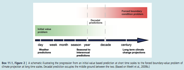
From IPCC AR5 Chapter 11
Figure 1
And in the introduction, chapter 1:
Climate in a narrow sense is usually defined as the average weather, or more rigorously, as the statistical description in terms of the mean and variability of relevant quantities over a period of time ranging from months to thousands or millions of years. The relevant quantities are most often surface variables such as temperature, precipitation and wind.
Classically the period for averaging these variables is 30 years, as defined by the World Meteorological Organization.
Climate in a wider sense also includes not just the mean conditions, but also the associated statistics (frequency, magnitude, persistence, trends, etc.), often combining parameters to describe phenomena such as droughts. Climate change refers to a change in the state of the climate that can be identified (e.g., by using statistical tests) by changes in the mean and/or the variability of its properties, and that persists for an extended period, typically decades or longer.
[Emphasis added].
Weather is an Initial Value Problem, Climate is a Boundary Value Problem
The idea is fundamental, the implementation is problematic.
As explained in Natural Variability and Chaos – Two – Lorenz 1963, there are two key points about a chaotic system:
- With even a minute uncertainty in the initial starting condition, the predictability of future states is very limited
- Over a long time period the statistics of the system are well-defined
(Being technical, the statistics are well-defined in a transitive system).
So in essence, we can’t predict the exact state of the future – from the current conditions – beyond a certain timescale which might be quite small. In fact, in current weather prediction this time period is about one week.
After a week we might as well say either “the weather on that day will be the same as now” or “the weather on that day will be the climatological average” – and either of these will be better than trying to predict the weather based on the initial state.
No one disagrees on this first point.
In current climate science and meteorology the term used is the skill of the forecast. Skill means, not how good is the forecast, but how much better is it than a naive approach like, “it’s July in New York City so the maximum air temperature today will be 28ºC”.
What happens in practice, as can be seen in the simple Lorenz system shown in Part Two, is a tiny uncertainty about the starting condition gets amplified. Two almost identical starting conditions will diverge rapidly – the “butterfly effect”. Eventually these two conditions are no more alike than one of the conditions and a time chosen at random from the future.
The wide divergence doesn’t mean that the future state can be anything. Here’s an example from the simple Lorenz system for three slightly different initial conditions:
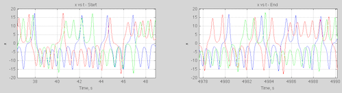
Figure 2
We can see that the three conditions that looked identical for the first 20 seconds (see figure 2 in Part Two) have diverged. The values are bounded but at any given time we can’t predict what the value will be.
On the second point – the statistics of the system, there is a tiny hiccup.
But first let’s review what is agreed upon. Climate is the statistics of weather. Weather is unpredictable more than a week ahead. Climate, as the statistics of weather, might be predictable. That is, just because weather is unpredictable, it doesn’t mean (or prove) that climate is also unpredictable.
This is what we find with simple chaotic systems.
So in the endeavor of climate modeling the best we can hope for is a probabilistic forecast. We have to run “a lot” of simulations and review the statistics of the parameter we are trying to measure.
To give a concrete example, we might determine from model simulations that the mean sea surface temperature in the western Pacific (between a certain latitude and longitude) in July has a mean of 29ºC with a standard deviation of 0.5ºC, while for a certain part of the north Atlantic it is 6ºC with a standard deviation of 3ºC. In the first case the spread of results tells us – if we are confident in our predictions – that we know the western Pacific SST quite accurately, but the north Atlantic SST has a lot of uncertainty. We can’t do anything about the model spread. In the end, the statistics are knowable (in theory), but the actual value on a given day or month or year are not.
Now onto the hiccup.
With “simple” chaotic systems that we can perfectly model (note 1) we don’t know in advance the timescale of “predictable statistics”. We have to run lots of simulations over long time periods until the statistics converge on the same result. If we have parameter uncertainty (see Ensemble Forecasting) this means we also have to run simulations over the spread of parameters.
Here’s my suggested alternative of the initial value vs boundary value problem:
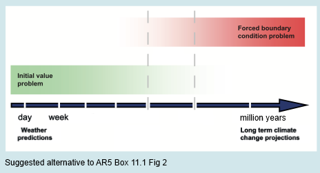
Figure 3
So one body made an ad hoc definition of climate as the 30-year average of weather.
If this definition is correct and accepted then “climate” is not a “boundary value problem” at all. Climate is an initial value problem and therefore a massive problem given our ability to forecast only one week ahead.
Suppose, equally reasonably, that the statistics of weather (=climate), given constant forcing (note 2), are predictable over a 10,000 year period.
In that case we can be confident that, with near perfect models, we have the ability to be confident about the averages, standard deviations, skews, etc of the temperature at various locations on the globe over a 10,000 year period.
Conclusion
The fact that chaotic systems exhibit certain behavior doesn’t mean that 30-year statistics of weather can be reliably predicted.
30-year statistics might be just as dependent on the initial state as the weather three weeks from today.
Articles in the Series
Natural Variability and Chaos – One – Introduction
Natural Variability and Chaos – Two – Lorenz 1963
Natural Variability and Chaos – Three – Attribution & Fingerprints
Natural Variability and Chaos – Four – The Thirty Year Myth
Natural Variability and Chaos – Five – Why Should Observations match Models?
Natural Variability and Chaos – Six – El Nino
Natural Variability and Chaos – Seven – Attribution & Fingerprints Or Shadows?
Natural Variability and Chaos – Eight – Abrupt Change
Notes
Note 1: The climate system is obviously imperfectly modeled by GCMs, and this will always be the case. The advantage of a simple model is we can state that the model is a perfect representation of the system – it is just a definition for convenience. It allows us to evaluate how slight changes in initial conditions or parameters affect our ability to predict the future.
The IPCC report also has continual reminders that the model is not reality, for example, chapter 11, p. 982:
For the remaining projections in this chapter the spread among the CMIP5 models is used as a simple, but crude, measure of uncertainty. The extent of agreement between the CMIP5 projections provides rough guidance about the likelihood of a particular outcome. But — as partly illustrated by the discussion above — it must be kept firmly in mind that the real world could fall outside of the range spanned by these particular models.
[Emphasis added].
Chapter 1, p.138:
Model spread is often used as a measure of climate response uncertainty, but such a measure is crude as it takes no account of factors such as model quality (Chapter 9) or model independence (e.g., Masson and Knutti, 2011; Pennell and Reichler, 2011), and not all variables of interest are adequately simulated by global climate models..
..Climate varies naturally on nearly all time and space scales, and quantifying precisely the nature of this variability is challenging, and is characterized by considerable uncertainty.
I haven’t yet been able to determine how these firmly noted and challenging uncertainties have been factored into the quantification of 95-100%, 99-100%, etc, in the various chapters of the IPCC report.
Note 2: There are some complications with defining exactly what system is under review. For example, do we take the current solar output, current obliquity,precession and eccentricity as fixed? If so, then any statistics will be calculated for a condition that will anyway be changing. Alternatively, we can take these values as changing inputs in so far as we know the changes – which is true for obliquity, precession and eccentricity but not for solar output.
The details don’t really alter the main point of this article.


On your suggested graph are some of the year marks missing as we aren’t sure what they are?
Ragnaar,
The marks in the original graphic relate to a specific question which is examined in Chapter 11 – about the possibility of decadal predictions and how initial values can assist this.
Once we consider the possibility that maybe “climate” – as long term statistics – might not be 10-100 years but instead 10,000 or 1,000,000 years averages, then this opportunity no longer exists.
I could have removed the marks, but I wasn’t so interested in the minutiae here.
I think there are many reasons why most ofcthe GCMs may not faithfully predict details of climate over intervals less than 100 years, but I also believI understand them well enough to say Lorenz style chaotic behavior isn’t one of them. They gave imperfections because the need for computational speed means some computations are in fact elaborate interpolations on tables of empirical values.
These models do not exhibit chaotic behavior when tested, rightly or wrongly.
I also think, saying with respect, that the figure of merit here may be a bit off. The key physical attributes they need to capture are GLOBAL and AVERAGE distributions of energy among subsystems, not for extreme instance, the number and size of cyclones that there’ll be in any paricylar year in say the north Atlantic. This is like the difference between considering a strictly Newtonian view of a mechanical system and contrasting it with a Hamiltonian description, in fact, *the* Hamiltonian.
There are plenty of simpler models which are physically based and have predictive skill at their level of resolution which don’t rely upon dynamical evolution of States. I refer the readership to those in Ray Pierrehumbert’s POPC for examples, as well as his computer codes. These are far more useful than Lorens philosophy.
Your suggested graph contain less year marks. Would say the IPCC’s graph overstated what is known about when the initial values/boundary values transition occurs?
‘The global coupled atmosphere–ocean–land–cryosphere system exhibits a
wide range of physical and dynamical phenomena with associated
physical, biological, and chemical feedbacks that collectively result
in a continuum of temporal and spatial variability. The traditional
boundaries between weather and climate are, therefore, somewhat
artificial.
The large-scale climate, for instance, determines the environment for
microscale (1 km or less) and mesoscale (from several kilometers to
several hundred kilometers) processes that govern weather and local
climate, and these small-scale processes likely have significant
impacts on the evolution of the large-scale circulation.’
James Hurrell, Gerald A. Meehl, David Bader, Thomas L. Delworth ,
Ben Kirtman, and Bruce Wielicki: A UNIFIED MODELING APPROACH TO CLIMATE SYSTEM PREDICTION, BAMS December 2009 | 1819: DOI:
10.1175/2009BAMS2752.1
At the scale of days weather is most obviously chaotic. At the scale of months to years we have this interim state that have been described as macro-weather. Beyond that are multi-decadal regimes with breakpoints identified at around 1912, the mid 1940’s, 1976/1977 and 1998/2002. These are synchronised changes in the Earth system seen in ocean and atmosphere indices and in the trajectory of surface temperatures.
Statistically a non-stationary system with changes in climate means and variance with a multi-decadal beat.
In the words of Michael Ghil (2013) the ‘global climate system is composed of a number of subsystems – atmosphere, biosphere, cryosphere, hydrosphere and lithosphere – each of which has distinct characteristic times, from days and weeks to centuries and millennia. Each subsystem, moreover, has its own internal variability, all other things being constant, over a fairly broad range of time scales. These ranges overlap between one subsystem and another. The interactions between the subsystems thus give rise to climate variability on all time scales.’
The theory suggests that the system is pushed by greenhouse gas changes and warming – as well as solar intensity and Earth orbital eccentricities – past a threshold at which stage the components start to interact chaotically in multiple and changing negative and positive feedbacks – as tremendous energies cascade through powerful subsystems. Some of these changes have a regularity within broad limits and the planet responds with a broad regularity in changes of ice, cloud, Atlantic thermohaline circulation and ocean and atmospheric circulation.
Dynamic climate sensitivity implies the potential for a small push to initiate a large shift. Climate in this theory of abrupt change is an emergent property of the shift in global energies as the system settles down into a new climate state. The traditional definition of climate sensitivity as a temperature response to changes in CO2 makes sense only in periods between climate shifts – as climate changes at shifts are internally generated. Climate evolution is discontinuous at the scale of decades and longer.
In the way of true science – it suggests at least decadal predictability. The current cool Pacific Ocean state seems more likely than not to persist for 20 to 40 years from 2002. The flip side is that – beyond the next few decades – the evolution of the global mean surface temperature may hold surprises on both the warm and cold ends of the spectrum (Swanson and Tsonis, 2009).
http://watertechbyrie.com/2014/06/23/the-unstable-math-of-michael-ghils-climate-sensitivity/
Models don’t exhibit chaotic behaviour?
Click to access 4751.full.pdf
http://www.pnas.org/content/104/21/8709.full
Can’t access the Total Sic article, but where in PNAS do they talk about chaotic behaviid? I Aldo don’t like the open ended and somewhat sloppy term “chaos”. I expect the deviation to be described in terms of aime Lyapuniv-like bound. That is, the norm of the M in
|y(t+d)-y(t)| = exp[M |x(t+d)-x(t)|]
You are obviously on your phone. Here’s the Royal Society article again – http://rsta.royalsocietypublishing.org/content/roypta/369/1956/4751.full
‘Lorenz was able to show that even for a simple set of nonlinear equations (1.1), the evolution of the solution could be changed by minute perturbations to the initial conditions, in other words, beyond a certain forecast lead time, there is no longer a single, deterministic solution and hence all forecasts must be treated as probabilistic. The fractionally dimensioned space occupied by the trajectories of the solutions of these nonlinear equations became known as the Lorenz attractor (figure 1), which suggests that nonlinear systems, such as the atmosphere, may exhibit regime-like structures that are, although fully deterministic, subject to abrupt and seemingly random change.’
What you expect and what you get may be two entirely different things. Are you really insisting that climate models are not chaotic?
(Apologies . Just catching up with what turned out to be a popular thread. And, yes, I was writing from my tablet, but unlike other Web sites, for some reason SoD kept wanting to return to the top of the Web page so I was typing blind.)
This response pertains to the comment “What you expect and what you get may be two entirely different things. Are you really insisting that climate models are not chaotic?”
There are three things.
First of all, as I believe I mentioned in another post last night, I believe, in dynamics, “chaos” is reserved for those situations where there is NO predictability at all. To use the Lyapunov setup I mentioned, actually, chaos would correspond to a situation where
|y(t+d) – y(t)| = exp[exp[exp[ … exp[|M(x(t+d) – x(t))|] …]]]
meaning that the change in output is arbitrarily sensitive to changes in input for a system y(t) = F(x(t)), and assuming non-trivial M. If there’s a different terminology for “chaos” used here, my pardons. If so, I’ll assume that “chaos” here is the lower order version I cited, that
|y(t+d) – y(t)| = exp[|M(x(t+d) – x(t))|]
meaning that the difference in output at different times is very sensitive to changes in difference of states, but not explosively so. In other words, predictability persists for a time, and then decays.
Second, there’s a distinction between the climate system in Nature, and climate models, which are descriptions of the former. One or both can exhibit “chaotic properties”. Whether Nature does or not is open to question here. As indicated, there are various coupled systems, each operating on different time scales, and even if it’s posited that one or more of these is chaotic, their different time scales and coupling suggested the behavior could be integrated away. Whether climate models do or not is a different question. Seen as a piece of numerical software, there are senses in which that software might exhibit “chaotic behavior”. But, then again, it may not. It depends upon the software.
Third, the meaning of whether or not “climate models” or even “climate” depends upon what’s precisely meant. A “climate observable” to me means a physical measurable or inferred parameter which is obtained by integrating over (averaging over, if you will) all “reasonable” initial states of the climate system for a period of evolution (or, if you will, of interest). If climate models are uncertain, it’s also sensible to talk about averaging over an indexed set of climate models to obtain an estimate of the measurable or parameter, although with uncertainty … In my preferred terms a posterior marginal density for the parameter.
Models have at their core a set of non-linear equations. Much as Lorenz’s convection model did. From there it is a modest step to the idea of sensitive dependence – perfectly deterministic but seemingly random in the words of Julia Slingo and Tim Palmer.
Or indeed James McWilliams.
‘Sensitive dependence and structural instability are humbling twin properties for chaotic dynamical systems, indicating limits about which kinds of questions are theoretically answerable. They echo other famous limitations on scientist’s expectations, namely the undecidability of some propositions within axiomatic mathematical systems (Gödel’s theorem) and the uncomputability of some algorithms due to excessive size of the calculation.’
http://www.pnas.org/content/104/21/8709.full
So these models are chaotic in the sense of complexity theory – and unless we get beyond mere definitional issues to the widespread understanding that it is so – then thee is nothing left to say.
Climate is chaotic – because it shifts abruptly. ‘What defines a climate change as abrupt? Technically, an abrupt climate change occurs when the climate system is forced to cross some threshold, triggering a transition to a new state at a rate determined by the climate system itself and faster than the cause. Chaotic processes in the climate system may allow the cause of such an abrupt climate change to be undetectably small.’ http://www.nap.edu/openbook.php?record_id=10136&page=14
Getting to an idea of what that means for the real system – is the problem.
‘‘Prediction of weather and climate are necessarily uncertain: our observations of weather and climate are uncertain, the models into which we assimilate this data and predict the future are uncertain, and external effects such as volcanoes and anthropogenic greenhouse emissions are also uncertain. Fundamentally, therefore, therefore we should think of weather and climate predictions in terms of equations whose basic prognostic variables are probability densities ρ(X,t) where X denotes some climatic variable and t denoted time. In this way, ρ(X,t)dV represents the probability that, at time t, the true value of X lies in some small volume dV of state space.’ (Predicting Weather and Climate – Palmer and Hagedorn eds – 2006)
Fundamentally – a probability density function of a family of solutions of a systematically perturbed model – rather than an ensemble of opportunity.
‘In each of these model–ensemble comparison studies, there are important but difficult questions: How well selected are the models for their plausibility? How much of the ensemble spread is reducible by further model improvements? How well can the spread can be explained by analysis of model differences? How much is irreducible imprecision in an AOS?
Simplistically, despite the opportunistic assemblage of the various AOS model ensembles, we can view the spreads in their results as upper bounds on their irreducible imprecision. Optimistically, we might think this upper bound is a substantial overestimate because AOS models are evolving and improving. Pessimistically, we can worry that the ensembles contain insufficient samples of possible plausible models, so the spreads may underestimate the true level of irreducible imprecision (cf., ref. 23). Realistically, we do not yet know how to make this assessment with confidence.’ http://www.pnas.org/content/104/21/8709.full
Whoa. That a model’s state at any particular time step is sensitively dependent upon initial conditions does not imply that a large-scale average of many many time steps’ worth of state (e.g., rolling 5-year GAT) is also sensitively dependent. That has yet to be shown.
I very much agree with you. I was just trotting out standard stuff about dynamical systems and chaos, not saying they applied to climate. I gave my doubts they do.
> So one body made an ad hoc definition of climate as the 30-year average of weather.
I don’t agree that its one body or particularly ad hoc, but I don’t think that’s your point, which appears to be:
> If this definition is correct and accepted then “climate” is not a “boundary value problem” at all. Climate is an initial value problem
I’m missing your leap of logic there. I could see that it is *possible* that in 30 year averages you could still be in the “weather” regime, and I’m sure you could construct systems in which that was true. But I don’t see where or how you’ve demonstrated the logical necessity of “climate is an IVP” following from “climate is 30y avg of weather”.
‘Technically, an abrupt climate change occurs when the climate system is forced to cross some threshold, triggering a transition to a new state at a rate determined by the climate system itself and faster than the cause. Chaotic processes in the climate system may allow the cause of such an abrupt climate change to be undetectably small…
Modern climate records include abrupt changes that are smaller and briefer than in paleoclimate records but show that abrupt climate change is not restricted to the distant past.’ (NAS, 2002)
You have to understand what is meant by an initial value problem in climate. A control variable pushes the system past a threshold at which stage internal processes interact to produce a different – emergent – climate state.
The resultant climate shift can be negative or positive – small or extreme. They happen every few decades – 20 to 40 years in the long proxy records.
I didn’t think there was ironclad evidence for big bifurcations in climate. In fact, I thought that, as of 2009 anyway, it was a serious computational challenge. See Simonnet, Dijkstra, Ghil, http://dspace.library.uu.nl/handle/1874/43777. Also thought that the mere existence of multiple equilibria in climate had not been established except for idealized versions, like aquaplanet (“Climate Determinism Revisited: Multiple Equilibria in a Complex Climate Model”), Ferreira, Marshall, Rose, http://journals.ametsoc.org/doi/abs/10.1175/2010JCLI3580.1. Equilibria need to exist to have bifurcations, even if they are unstable. If by “bifurcations” is meant transitions between states which are not siginificantly separated, then I wonder if they deserve the term “bifurcation”.
BTW, on the matter of climate bifurcations, I put to Professor Marshall something I read here, probably in a discussion of bifurcations in a comment thread pertaining to initiation of ice ages, that evidence was state transitions happened slowly if there were multiple equilibria. I am, of course, quoting him and could have gotten something wrong, but my understanding of his response was that if multiple equilibria existed, there was no particular physical reason to believe that transitions between them would necessarily take a long time.
‘Technically, an abrupt climate change occurs when the climate system is forced to cross some threshold, triggering a transition to a new state at a rate determined by the climate system itself and faster than the cause. Chaotic processes in the climate system may allow the cause of such an abrupt climate change to be undetectably small…
Modern climate records include abrupt changes that are smaller and briefer than in paleoclimate records but show that abrupt climate change is not restricted to the distant past.’ (NAS, 2002)
I quote this again. Abrupt change in the climate system – evident everywhere and at all scales – is what is explained by complexity theory. Really it is just the result of the interactions of system components.
The theory suggests that the system is pushed by greenhouse gas changes and warming – as well as solar intensity and Earth orbital eccentricities – past a threshold at which stage the components start to interact chaotically in multiple and changing negative and positive feedbacks – as tremendous energies cascade through powerful subsystems. Some of these changes have a regularity within broad limits and the planet responds with a broad regularity in changes of ice, cloud, Atlantic thermohaline circulation and ocean and atmospheric circulation.
“The winds change the ocean currents which in turn affect the climate. In our study, we were able to identify and realistically reproduce the key processes for the two abrupt climate shifts,” says Prof. Latif. “We have taken a major step forward in terms of short-term climate forecasting, especially with regard to the development of global warming. However, we are still miles away from any reliable answers to the question whether the coming winter in Germany will be rather warm or cold.” Prof. Latif cautions against too much optimism regarding short-term regional climate predictions: “Since the reliability of those predictions is still at about 50%, you might as well flip a coin.” http://www.sciencedaily.com/releases/2013/08/130822105042.htm
Realistically – you may as well flip a coin. But it is conceptually a better description of reality.
William,
It is my point.
A “typical simple” chaotic system has a timescale over which the statistics are repeatable.
I’m making the reasonable claim that for our climate this timescale is not 30 years. If someone wants to demonstrate that it is, I look forward to the evidence.
The “classical case” that climate is the 30 year statistics of weather was not concluded on the basis of some discovery on the nature of climate as a chaotic system.
Until you reach the timescale for repeatable statistics you are in a zone where small differences in initial values result in divergences that are as significant as the differences between two randomly selected states.
That is, unpredictable.
Let me be clear that I can’t prove that the repeatable statistics of weather are reached over 10,000 year periods either. It might be 300,000 years or 10,000,000 years.
Grant you, and as I suggested elsewhere, “disaster in Canberra” might be unpredictable, but, as I also suggested elsewhere, the World Line of Earth is only one of many possible statistical realizations from Now. And I think the domain and claim of models is that while it may be very difficult/impossible to pick out which World Line will be followed, the properties of the global state at some future time are far more stable, and decent confidence bounds can be given. It’s not like there’s a possibility of Runaway Greenhouse or Snowball Earth in the range of likelihoods, which seems to be the implication of this argument.
Sorry, I don’t buy categorical “unpredictability”. I buy a hierarchy of probable outcomes.
Another possibility is that the “attractor” for weather statistics is, from our point of view, quite limited in range. If that is the case, then even though we don’t know the result on a given day/month/year/decade – we would know that the results were confined to a small set of values.
Again, that idea would need to be demonstrated.
The point of this article is to show the divide between an arbitrary set of statistics and the long term statistics of a chaotic system.
It’s not science to conflate the two without evidence.
if we argue that the climate system is chaotic in some sense(s), we must then describe the region(s) over which chaos significantly affects the climate’s state. Where are the boundaries? Clearly there are some established by basic thermodynamics: e.g., GAT will not reach 400K under current forcings. The clear responses to diurnal and annual forcings further shrink the possible chaotic region(s), as do (to a lesser extent) analyses of the response to volcanic forcing (e.g., Pinatubo’s ~2.5W/m^2 SW forcing over ~2 y causing a ~0.25C drop in GAT over that period).
So where are the boundaries? What is the hypothesis of chaotic climate, and how can we test its predictions?
Meow,
It’s perhaps a little different from the way you are looking at the problem.
Let’s take a typical (dissipative) chaotic system, like the well-known Lorenz 1963 system, as an example.
There are 3 parameters, x = intensity of convection, y = temperature difference between ascending and descending currents, z = deviation of temperature from a linear profile
Here is how x varies at certain periods, the colors relate to a few very slightly different initial conditions (this figure was shown in the article):
The key points are that:
1. there are boundaries – we can see that x is constrained to certain values regardless of where we are in the timeline
2. these boundaries of x are defined by the equations of the system – and, therefore, the parameters in the equations
3. the long term statistics (of which the “boundaries” are just one statistic) are reliable
4. predicting the actual value of x at any given time is impossible
It’s not a case of which bit is due to the “forcing” and which bit is due to the “chaos”.
The statistics of x,y,x will be moved around by changing the parameters (or the form of the equation). The values of x,y,z at a specific time will be unknown. The statistics of x,y,x will be known.
So for example (given a model which perfectly reproduces the physics), given the parameters of the equation we can state at any given time the probability of x being in any given range.
If the “forcing” changes, this will change the statistics. The future value at a specific time will still be unknowable. The future statistics will be knowable.
In the case of the Lorenz system we can change the forcing by changing the parameter r. The statistics change.
Of course, in this simple system reducing r to a certain value takes us out of the chaotic region.
Increasing r to a certain value takes us out of the chaotic region.
It isn’t about saying which bit is due to chaos. Chaos never means unbounded possibility.
Chaos means that a given value can be anywhere on the “attractor”, but nowhere else. (More precisely, it can start somewhere else but will always end up on the attractor).
The attractor is just a name for the “set of possible values for the parameter”.
Change the “forcing” – or a parameter – and you change the attractor.
Thank you for the explanation. Perhaps my question should be restated as: how does the hypothesis of chaotic climate account for the effects of known forcings (e.g., annual)? Or: how large must a forcing be for us to enter the realm where we reasonably can predict the resulting change in GAT or ocean heat content? (I don’t, of course, mean by this “predict an exact value on a given day”, but rather something like “predict a yearly or multi-yearly average with reasonable confidence”).
Meow,
I’m not sure I understand the question.
I don’t know.
Simple chaotic systems have boundaries so you know that certain values will be within certain limits. Under one time period you have no ability to predict the statistics, only that the value will be inside this range. Over a longer time period you have ability to predict the statistics – mean, standard deviation, etc.
There is no a priori reason to expect that this “longer time period” is “multi-year” (where I assume from the way you write “multi-year” you mean like 10 years or something, not 100,000 years).
There’s a further complication that I will spend more time on a subsequent article – in brief, because of the complexity of the climate system the boundary of entire climate states is probably exceptionally large, but in particular periods the boundary of entire climate states will be a lot smaller.
But clearly the length of the time period over which some climate statistics become reasonably predictable is inversely correlated to the integrated magnitude of a postulated forcing. If TSI were to fall by 50% and stay there, all of us would predict a sudden, large drop in GAT.
What I’m trying to do is to understand the shape of the forcing magnitude/predictability horizon curve, and, more broadly, the testable predictions of the hypothesis of chaotic climate. I must admit to being skeptical that the characteristics of the Lorenz model have much to do with large-scale climate statistics like GAT or OHC.
There has been much interesting research on climate predictability, which I hope you’ll get into. A few papers that stand out are Shukla 1998, “Predictability in the Midst of Chaos: A Scientific Basis for Climate Forecasting”, http://w.monsoondata.org/people/Shukla%27s%20Articles/1998/Predictability.pdf , and Goddard et al 2001, “Current Approaches to Seasonal-to-Internannual Climate Predictions”, http://onlinelibrary.wiley.com/doi/10.1002/joc.636/abstract .
BTW, thank you for publishing this site. It is an excellent resource.
If “the repeatable statistics of weather are reached” over a longer-than-150-year period, there is no practical application for climate models as yet.
‘We construct a network of observed climate indices in the period 1900–2000 and investigate their collective behavior. The results indicate that this network synchronized several times in this period. We find that in those cases where the synchronous state was followed by a steady increase in the coupling strength between the indices, the synchronous state was destroyed, after which a new climate state emerged. These shifts are associated with significant changes in global temperature trend and in ENSO variability. The latest such event is known as the great climate shift of the 1970s. We also find the evidence for such type of behavior in two climate simulations using a state-of-the-art model. This is the first time that this mechanism, which appears consistent with the theory of synchronized chaos, is discovered in a physical system of the size and complexity of the climate system.’ http://onlinelibrary.wiley.com/doi/10.1029/2007GL030288/full
Climate chaos is ergodic over long periods – perhaps. What matters more is the statistically non-stationary abrupt shifts in climate states at decadal to millennial scales of variability. It is a new way of thinking about climate as a system rather than as disparate parts. As Marcia Wyatt said – climate ‘is ultimately complex. Complexity begs for reductionism. With reductionism, a puzzle is studied by way of its pieces. While this approach illuminates the climate system’s components, climate’s full picture remains elusive. Understanding the pieces does not ensure understanding the collection of pieces.’ Understanding climate begins by viewing it through the lens of complexity theory.
The US National Academy of Sciences (NAS) defined abrupt climate change as a new climate paradigm as long ago as 2002. A paradigm in the scientific sense is a theory that explains observations. A new science paradigm is one that better explains data – in this case climate data – than the old theory. The new theory says that climate change occurs as discrete jumps in the system. Climate is more like a kaleidoscope – shake it up and a new pattern emerges – than a control knob with a linear gain.
The theory of abrupt climate change is the most modern – and powerful – in climate science and has profound implications for the evolution of climate this century and beyond. A mechanical analogy might set the scene. The finger pushing the balance below can be likened to changes in greenhouse gases, solar intensity or orbital eccentricity. The climate response is internally generated – with changes in cloud, ice, dust and biology – and proceeds at a pace determined by the system itself. Thus the balance below is pushed past a point at which stage a new equilibrium spontaneously emerges. Unlike the simple system below – climate has many equilibria. The old theory of climate suggests that warming is inevitable. The new theory suggests that global warming is not guaranteed and that climate surprises are inevitable.
Many simple systems exhibit abrupt change. The balance above consists of a curved track on a fulcrum. The arms are curved so that there are two stable states where a ball may rest. ‘A ball is placed on the track and is free to roll until it reaches its point of rest. This system has three equilibria denoted (a), (b) and (c) in the top row of the figure. The middle equilibrium (b) is unstable: if the ball is displaced ever so slightly to one side or another, the displacement will accelerate until the system is in a state far from its original position. In contrast, if the ball in state (a) or (c) is displaced, the balance will merely rock a bit back and forth, and the ball will roll slightly within its cup until friction restores it to its original equilibrium.’(NAS, 2002)
In (a1) the arms are displaced but not sufficiently to cause the ball to cross the balance to the other side. In (a2) the balance is displaced with sufficient force to cause the ball to move to a new equilibrium state on the other arm. There is a third possibility in that the balance is hit with enough force to cause the ball to leave the track, roll off the table and under the sofa.
“Climate chaos is ergodic over long periods”. What the heck does *that* mean?
First, I continue to ask for a mathematical definition of “climate chaos”. As far as I know, none has been provided.
Second, generally speaking, “ergodic” means, among other things, every state in the system under consideration will in time be visited. No one has demonstrated anything of the kind for the Earth’s climate, Mars climate, Venus’ climate, climate models, or anything else. Why should it be plausible for this magical “climate chaos”?
The full sentence was – climate chaos is ergodic over long periods – perhaps. It was an ironic restatement of the premise of the post – and getting all uppity about it is quite tedious. Not quoting the entire sentence smacks of bad faith.
Ergodic is this sense is as you say – and there is no ergodic theory of spatio-temporal chaotic systems. Hence the qualifier – perhaps.
You may ‘continually ask’ – but what you ask for is not necessarily what you will get – as I said. As there are no concise governing equations for the climate system – a mathematical treatment of the evolution of those equations – a la Poincare’s three body problem or Lorenz’s convection model – may be a trifle unrealistic.
Have I quoted Julia Slingo and Tim Palmer yet?
‘Lorenz was able to show that even for a simple set of nonlinear equations (1.1), the evolution of the solution could be changed by minute perturbations to the initial conditions, in other words, beyond a certain forecast lead time, there is no longer a single, deterministic solution and hence all forecasts must be treated as probabilistic. The fractionally dimensioned space occupied by the trajectories of the solutions of these nonlinear equations became known as the Lorenz attractor (figure 1), which suggests that nonlinear systems, such as the atmosphere, may exhibit regime-like structures that are, although fully deterministic, subject to abrupt and seemingly random change.’
http://rsta.royalsocietypublishing.org/content/roypta/369/1956/4751.full
Abrupt and seemingly random seem to be the crux of the magic.
It may be the “crux of the magic”, but, as I’ve contended, it’s horrible science, unfalsifiable. Chaos theory applied to climate is like string theory applied to the universe.
Sure it’s falsifiable. Produce a numerical weather model that will forecast the local weather with good skill two months in advance. Then I’ll believe that weather isn’t chaotic. Chaos theory tells you what questions it’s pointless to ask.
That’s not a falsification of the Chaos hypothesis, because the Chaos hypothesis is not making any predictions. To the degree it doesn’t, it can’t be used as a guide for doing science.
But, to your point, would it also be falsified if sea level in 400 years were at least 65 feet above present day?
It’s obviously the same prediction you get from ‘cycles’ – but the mechanism is dynamical complexity.
But the comment about skill put me in mind of another footnote from James McWilliams.
‘Sensitive dependence and structural instability are humbling twin properties for chaotic dynamical systems, indicating limits about which kinds of questions are theoretically answerable. They echo other famous limitations on scientist’s expectations, namely the undecidability of some propositions within axiomatic mathematical systems (Gödel’s theorem) and the uncomputability of some algorithms due to excessive size of the calculation.’
Let me expand a little – and then I think I will give it a rest. I have quoted Michael Ghil – but will repeat for convenience. The ‘global climate system is composed of a number of subsystems – atmosphere, biosphere, cryosphere, hydrosphere and lithosphere – each of which has distinct characteristic times, from days and weeks to centuries and millennia. Each subsystem, moreover, has its own internal variability, all other things being constant, over a fairly broad range of time scales. These ranges overlap between one subsystem and another. The interactions between the subsystems thus give rise to climate variability on all time scales.’
I have also shown a graph below from Kyle Swanson at realclimate showing warming resuming around 2020. The regimes are more like 20 to 40 years in the long proxy records – and the paper says it is an indeterminate period.
So the suggestion is that the current lack of surface warming – or even cooling – will persist for 20 to 40 years from 2002. The system will then abruptly shift to a new state involving a new trend in surface temperature and a change in the frequency and intensity of ENSO events in particular. These are abrupt changes from interactions of components – and not slow changes due to the evolution of forcing.
The specific decadal changes in ENSO can be eyeballed. Blue dominant to 1976 – red to 1998 and blue again since.
Something to think about is the millennial high point in El Nino frequency in the 20th century. More salt in the Law Dome ice core is La Nina.
Imprecise predictions seems a better bet than precise predictions that are utterly wrong.
Insufficient information.
I mean, such a prediction regarding SLR can be made simply by looking at the historical record, without appeal to “climate models”. In this case, the last time atmospheric CO2 was 400 ppm SLR was +65 feet more than now, so, one would estimate, after equilibration, that’s where they’ll end up now. If manifestations in climate are “chaotic”, SLR might be 65 feet or it might not be. There is no historical or archaeological record suggesting seas have been 65 feet higher, at least since the Iron Age, so a prediction of SLR +65 feet is truly extraordinary. So, I ask again, what does this “emerging” science of climate chaos say about this? In contrast, such a prediction *is* available from at least *some* climate models being maligned here.
“So one body made an ad hoc definition of climate as the 30-year average of weather.”
I can’t see the point you are making – who defined “climate” as a 30-year average of weather?
My understanding is the various meteorological bodies use 30 years as a convention for getting meaningful trends out of noisy data ie bringing the signal to noise ratio down to acceptable levels.
No one is saying there is anything special about 30 years.
The WMO.
[emphasis added]
Phil Jones on the origins of the ’30 years is climate’ —
From: Phil Jones
To: “Parker, David (Met Office)” , Neil Plummer
Subject: RE: Fwd: Monthly CLIMATbulletins
Date: Thu Jan 6 08:54:58 2005
Cc: “Thomas C Peterson”
Neil,
Just to reiterate David’s points, I’m hoping that IPCC will stick with 1961-90.
The issue of confusing users/media with new anomalies from a
different base period is the key one in my mind. Arguments about
the 1990s being better observed than the 1960s don’t hold too much
water with me.
There is some discussion of going to 1981-2000 to help the modelling
chapters. If we do this it will be a bit of a bodge as it will be hard to do
things properly for the surface temp and precip as we’d lose loads of
stations with long records that would then have incomplete normals.
If we do we will likely achieve it by rezeroing series and maps in
an ad hoc way.
There won’t be any move by IPCC to go for 1971-2000, as it won’t
help with satellite series or the models. 1981-2000 helps with MSU
series and the much better Reanalyses and also globally-complete
SST.
20 years (1981-2000) isn’t 30 years, but the rationale for 30 years
isn’t that compelling. The original argument was for 35 years around
1900 because Bruckner found 35 cycles in some west Russian
lakes (hence periods like 1881-1915). This went to 30 as it
easier to compute.
Personally I don’t want to change the base period till after I retire !
Cheers
Phil
Robert,
This is more about baselines for describing anomalies. You could set it to an arbitrary value, the value for one year, the average over 20 years, 50 years. Changing the baselines can create a lot of work. Different groups using different baselines creates lots of work in comparisons.
The “definition” of climate as the statistics of weather over 30 years is much older than this email.
“No one disagrees on this first point.”
I do, follow the links to a forecast for late 2015 to early 2017:
The article was talking about the prediction of weather using models. Not about predicting the weather using astrology.
The dynamics of the Earth system includes mechanisms that operate over a large range of time scales.
Purely atmospheric phenomena operate on the shortest time scale up to weeks. Beyond that variations in the state of the ocean starts to dominate for the expectation, and we do not really know what’s the maximum period over which the oceans have memory that leads to significant unforced variability. Perhaps the multidecadal oscillations of a quasiperiod of around 60 years are significant, while nothing beyond that it important, but that’s only one possibility. Some think that unforced variability is weak even on this time scale, while others may propose that similar phenomena occur also over longer periods asking whether MWP and LIA were as strong as higher estimates tell and mostly unforced.
Looking at much longer periods we have the question on the nature of the glacial cycles of around 100,000 years. Is that mainly controlled by internal dynamics of external (Milankovic) forcing? And what about the whole range of time scales between 100 y and 100,000 y?
The internal variability has both causal dependence on initial values and effectively chaotic components on all time scales. Something is predictable, in principle, on every time scale, while something else is not. As one example we have on the time scale of few years some initial value dependence in ENSO, and through that in weather, while we cannot make forecasts that specify further the weather of a given day in 2015.
Stating values like 30 years for what’s climate makes sense only as a way of assuring that short term variability is averaged away. If we could observe an ensemble of parallel universes that have the same forcings, we could define climate even for a single day, but lacking that possibility our possibilities of observing climate are limited to longer periods. No single length of the period has any unique status. 30 years is just one possible choice with some advantages and some disadvantages.
‘”The ocean plays a crucial role in our climate system, especially when it comes to fluctuations over several years or decades,” explains Prof. Mojib Latif, co-author of the study. “The chances of correctly predicting such variations are much better than the weather for the next few weeks, because the climate is far less chaotic than the rapidly changing weather conditions,” said Latif. This is due to the slow changes in ocean currents which affect climate parameters such as air temperature and precipitation. “The fluctuations of the currents bring order to the weather chaos”. http://www.geomar.de/en/news/article/klimavorhersagen-ueber-mehrere-jahre-moeglich/
Latif is not perhaps a little imprecise in his language. These abrupt changes in ocean and atmospheric in 1976/77 and 1998/2002 he is discussing are chaotic – merely on a longer scale.
Anastasios Tsonis, of the Atmospheric Sciences Group at University of Wisconsin, Milwaukee, and colleagues used a mathematical network approach to analyse abrupt climate change on decadal timescales. Ocean and atmospheric indices – in this case the El Niño Southern Oscillation, the Pacific Decadal Oscillation, the North Atlantic Oscillation and the North Pacific Oscillation – can be thought of as chaotic oscillators that capture the major modes of climate variability. Tsonis and colleagues calculated the ‘distance’ between the indices. It was found that they would synchronise at certain times and then shift into a new state.
It is no coincidence that shifts in ocean and atmospheric indices occur at the same time as changes in the trajectory of global surface temperature. Our ‘interest is to understand – first the natural variability of climate – and then take it from there. So we were very excited when we realized a lot of changes in the past century from warmer to cooler and then back to warmer were all natural,’ Tsonis said.
Four multi-decadal climate shifts were identified in the last century coinciding with changes in the surface temperature trajectory. Warming from 1909 to the mid 1940’s, cooling to the late 1970’s, warming to 1998 and – at the least – little warming since. There are practical implications for disentangling natural from anthropogenic change in recent climate. Using 1994 to 1998 – for instance – to average climate over a full cool and warm regime. Instead of an arbitrary starting point of 1950.
Sorry for you that the signals in Hayes’ and Imbries’ sediment cores, with frequencies of ~23, ~42 and ~100 k years matching precession, obliquity and eccentricity, do not support your theories on ‘climate surprises’. In contrast to SoD, you should not put the 1976 paper of Hayes et al. on top of your theoretical papers. You should read it first.
Seeing as we are delving into scientific pre-history – perhaps you should try – http://web.vims.edu/sms/Courses/ms501_2000/Broecker1995.pdf
Milankovich cycles set the conditions for persistence of ice and snow feedbacks – due to low NH summer insolation – that are initiated by changes in thermohaline circulation. The physical principles are feedbacks in a chaotic system.
In the words of Michael Ghil (2013) the ‘global climate system is composed of a number of subsystems – atmosphere, biosphere, cryosphere, hydrosphere and lithosphere – each of which has distinct characteristic times, from days and weeks to centuries and millennia. Each subsystem, moreover, has its own internal variability, all other things being constant, over a fairly broad range of time scales. These ranges overlap between one subsystem and another. The interactions between the subsystems thus give rise to climate variability on all time scales.’
The theory suggests that the system is pushed by greenhouse gas changes and warming – as well as solar intensity and Earth orbital eccentricities – past a threshold at which stage the components start to interact chaotically in multiple and changing negative and positive feedbacks – as tremendous energies cascade through powerful subsystems. Some of these changes have a regularity within broad limits and the planet responds with a broad regularity in changes of ice, cloud, Atlantic thermohaline circulation and ocean and atmospheric circulation.
The orbital eccentricities are not forcing as such but control variables in a chaotic system.
The paradigm emerges from observation of abrupt changes in the Earth system – such as is not explained by (relatively) smoothly evolving orbits.
‘Recent scientific evidence shows that major and widespread climate changes have occurred with startling speed. For example, roughly half the north Atlantic warming since the last ice age was achieved in only a decade, and it was accompanied by significant climatic changes across most of the globe. Similar events, including local warmings as large as 16°C, occurred repeatedly during the slide into and climb out of the last ice age. Human civilizations arose after those extreme, global ice-age climate jumps. Severe droughts and other regional climate events during the current warm period have shown similar tendencies of abrupt onset and great persistence, often with adverse effects on societies.’ Abrupt climate change: inevitable surprises – NAS 2002
As as reference to cite proof, Tsonis and colleague Swanson are tricky, since they tend to redefine terms like “random variable” from that taught in basic probability courses to, I would argue, less useful definitions in terms of computer programs. See http://onlinelibrary.wiley.com/doi/10.1029/2004EO380002/pdf.
Also, I would argue, a purely classical approach to climate series — or any series, for that matter — devoid of underlying physics, is limited by the accuracies of the represented series. In particular, I note, in little of the work reported, are uncertainties of individual by-year points included to weight the results. Surely, these *are* available.
Don’t forget Sergey Kravtsov. The great breakthrough of Tsonis and colleagues was the use real world data in a network model to demonstrate synchronous chaos in the Earth system. These indices were considered as chaotic oscillating nodes on a network and the resultant timing of synchonisation identified. That it is also the inflection points of global surface temperature – and of global hydrology – says that real connections were identified.
It is very much a systems approach that stimulated the development of the stadium wave idea of Marcia Wyatt and – latterly – Judith Curry. It is very much about the evolution of the Earth system as a whole.
.
I remembered this one – talking about the underlying physics Tsonis is aiming at.
Click to access PhysicaD.pdf
In “Emergence of synchronization in complex networks of interacting
dynamical systems”, theory is fine, and networks of coupled oscillators are interesting and fine, but apart from fitting these to a few series, what do they have to do with climate science? Moreover, since the approach is frequentist, where in this work are the corrections for overfitting?
Anastasios Tsonis, of the Atmospheric Sciences Group at University of Wisconsin, Milwaukee, and colleagues used a mathematical network approach to analyse abrupt climate change on decadal timescales. Ocean and atmospheric indices – in this case the El Niño Southern Oscillation, the Pacific Decadal Oscillation, the North Atlantic Oscillation and the North Pacific Oscillation – can be thought of as chaotic oscillators that capture the major modes of NH climate variability. Tsonis and colleagues calculated the ‘distance’ between the indices. It was found that they would synchronise at certain times and then shift into a new state.
‘The distance can be thought as the average correlation between all possible pairs of nodes and is interpreted as a measure of the synchronization of the network’s components. Synchronization between nonlinear (chaotic) oscillators occurs when their corresponding signals converge to a common, albeit irregular, signal. In this case, the signals are identical and their cross-correlation is maximized. Thus, a distance of zero corresponds to a complete synchronization and a distance of the square root of 2 signifies a set of uncorrelated nodes.’ http://onlinelibrary.wiley.com/doi/10.1029/2007GL030288/full
These indices are physical realities with major effects on global hydrology. – e.g.
That behave very much like chaotic oscillators at various scales. The method attempts to see how these are linked in a global networked system. A whole new approach – a new way of looking at these things – hence the title of the paper.
https://hypergeometric.wordpress.com/2014/12/01/tsonis-swanson-chaos-and-s__t-happens/
‘First, there is no instance where their series based explanation makes a prediction that is falsifiable. I challenge them to make one.’
‘Second, while they offer a statistical explanation of series, they have not advanced a physical mechanism for its realization, something essential for both taking it seriously as a hypothesis and for supporting additional scientific work based upon it. They can’t say what additional measurements are to be taken or where. Indeed, from their perspective, doing additional measurements is somewhat pointless. due to the “chaotic” nature of outcomes.’
Three great physical theories emerged in the 20th century – relativity, quantum mechanics and chaos. The letter is the theory of complex and dynamic systems. The expectation of the behaviour of these systems include an increase in autocorrelation (e.g http://www.pnas.org/content/105/38/14308.full) and noisy bifurcation (e.g. http://arxiv.org/abs/0907.4290). It is all completely deterministic – but ultimately too complex to determined completely as yet.
‘Third, they embrace the popular understanding of “chaos” from the Lorenz setting rather than a technical one, so the scientific reader really doesn’t know from paragraph to paragraph what exactly they are talking about.’
I certainly don’t agree. Perhaps related (to non-linearities in climate) reading first might help.
e.g. http://www.fraw.org.uk/files/climate/rial_2004.pdf
There is first of all the fact of abrupt change – at decadal scales even – in the climate system. Then there is a paradigm that explains the observations. The US National Academy of Sciences (NAS) defined abrupt climate change as a new climate paradigm as long ago as 2002. A paradigm in the scientific sense is a theory that explains observations. A new science paradigm is one that better explains data – in this case climate data – than the old theory. The new theory says that climate change occurs as discrete jumps in the system. Climate is more like a kaleidoscope – shake it up and a new pattern emerges – than a control knob with a linear gain. .
Regarding definitions of “chaos”, I was simply going back to dynamical systems work which originated the concept. It doesn’t matter whether or not NAS used the term, or some peer-reviewed publication used the term, any more than poor use of t-tests appear in climate, meteorological, or physical literature. Poor use of t-tests is done in medical literature all the time. There is no definition of “chaos”. There are only grades. The chaotic pendulum where the predictive response is the number of times the pendulum rotates about the mount before settling back in the well has a spectrum of behaviors, depending upon impulse of launching it. Where *exactly* is the chaotic boundary? There isn’t one! “Chaos” refers to the phenomenon that in some region of impulse, the prediction of the number of rotates before settling back into the energy well are less and less uncertain. But they aren’t *inherently* uncertain! Start modeling the frictive forces, per tribology, and predictions become sharper.
Regarding ” A new science paradigm is one that better explains data – in this case climate data – than the old theory”, I disagree. “Better explains” is more than being logically consistent. “Better explains” means *predicting* with smaller error bars. In this case, a “better hypothesis” would need to hindcast and forecast with smaller error bars. The “chaotic theory” gives up on being able to do that. That’s one reason why, in another place, I say it’s “not even wrong”.
‘AOS models are members of the broader class of deterministic chaotic dynamical systems, which provides several expectations about their properties (Fig. 1). In the context of weather prediction, the generic property of sensitive dependence is well understood (4, 5). For a particular model, small differences in initial state (indistinguishable within the sampling uncertainty for atmospheric measurements) amplify with time at an exponential rate until saturating at a magnitude comparable to the range of intrinsic variability. Model differences are another source of sensitive dependence. Thus, a deterministic weather forecast cannot be accurate after a period of a few weeks, and the time interval for skillful modern forecasts is only somewhat shorter than the estimate for this theoretical limit. In the context of equilibrium climate dynamics, there is another generic property that is also relevant for AOS, namely structural instability (6). Small changes in model formulation, either its equation set or parameter values, induce significant differences in the long-time distribution functions for the dependent variables (i.e., the phase-space attractor). The character of the changes can be either metrical (e.g., different means or variances) or topological (different attractor shapes). Structural instability is the norm for broad classes of chaotic dynamical systems that can be so assessed (e.g., see ref. 7).’ http://www.pnas.org/content/104/21/8709.full
The original dynamic analysis was Poincaré’s 3 body problem.
http://www.upscale.utoronto.ca/GeneralInterest/Harrison/Flash/Chaos/ThreeBody/ThreeBody.html
Chaos is in the sudden shifts in trajectory between the attractor basins that comprise the solution space for the equations.
The idea lay dormant for 60 years until it was rediscovered in Lorenz’s set of non-linear equations. It has since been extended to a ‘broader class’ of dynamical systems in applications ranging from ecology to economics. As James McWilliams says in the quote – there are expectations about their behaviour.
SoD,
whenever I have to think about chaos theory, the first thing I always do is to pick up a copy of the old paper from Hays, Imbrie and Shackleton (1976) on obliquity and precession and to put it on top of the stack of papers on chaos theory. It’s the perfect antidote against loosing ground amongst strange attractors (which, I fear, happens to you right now). Forced, predictable responses are not something you get only in the output of climate models. They are real. They are imprinted in almost any climate archive. Don’t forget them.
The orbital parameters set conditions for ice and snow feedbacks Think abrupt change rather than chaos.
verbascose,
I suggest you read the series here Ghosts of Climates Past (part 1 here). I don’t think you will look at Hays, Imbrie and Shackleton (1976) (see part 3) quite the same afterwards.
Nope, doesn’t change anything. My point here is solely empirical: there are these frequencies in the sediment cores (and in many other climate archives as well). If chaotic processes would dominate and would be able to override forced responses with ease, one would not find regular patterns in cores.
verbascose,
If the chaotic behavior of the climate system were not able to override forced responses, the period of glacial/interglacial transitions would still be ~40ky. The signal from eccentricity at 100ky is simply not strong enough to explain this change in period. Not to mention that the most recent transitions do not, in fact, correlate with eccentricity. Then there is also the circularity of the dating of ocean cores, and hence glacial/interglacial transitions, by using Milankovitch cycles. In logic, that’s called begging the question.
As SoD points out, you need more than a hypothetical mechanism. You have to show that the mechanism works. That hasn’t been accomplished so far.
verbascose,
I’m not claiming that they “override forced responses with ease”, or even that they “override forced responses”.
What is the time period between the last 4 ice age terminations? It’s not 100kyrs.
I did a calculation based on one set of dates:
I-II = 124 kyrs
II-III = 111
III-IV = 86
IV-V = 79
V-VI = 102
Peter Huybers & Carl Wunsch came up with probably one of the best theories, which is that ice age terminations are paced by obliquity, i.e. they occur in multiples of 40kyrs. That’s how strong the 100kyr theory is!
Obliquity pacing of the late Pleistocene glacial terminations, Huybers & Wunsch, Nature (2005):
Of course, there are other models. A recent one, also published in Nature, by Abe-Ouchi uses an ice sheet model, with the hysteresis of the isostatic rebound being a big part of the terminations.
Insolation-driven 100,000-year glacial cycles and hysteresis of ice-sheet volume, Ayako Abe-Ouchi et al, Nature (2013)
Verbascose: Are you an emerging prebiotic?
http://pubchem.ncbi.nlm.nih.gov/compound/Verbascose#section=Top
Click to access Casey-Johnson-Lentils-A-Prebiotic-Rich-Whole-Food-for-Reducing-Obesity-and-NCDs.pdf
If so, cool. Thanks for kicking up dust and creating interesting reading.
WRT the main topic:
Looking at the 5.5MY temperature record
http://en.wikipedia.org/wiki/Geologic_temperature_record
It appears that since the Pliocene closure of Panama (and the Atlantic becoming a type of Chua’s circuit) the ~100K cycles represent the onset of dynamic equilibrium. Therefore, an equatorial oceanic block is a *forcing* that shifts the climate to a new plateau in ~2MY. The current tectonic climate configuration appears to be ~100K +/- 33%. The 40K cycle is damped by the land ice-sea ice-ocean system.
Blame the Great Lakes
As the temperature continued to drop from 3 to 1-MY, the scoured out Ice Sheet along the Great Lakes basin made roots that allowed for greater ice thickness, massive buildup and reduced linear flow to calving.
A Land-Ice Bubble.
The Ice Sheets became *Too Big To Fail* surviving multiple DO events pushing past the previous 41K limits, then crashed from their immense mass coated with teratons of dust from an increasing dry and exposed crust.
Is that Chaos?
verbascose,
I reviewed the opinions of climate scientists on ice age terminations in Ghosts of Climates Past – Eighteen – “Probably Nonlinearity” of Unknown Origin.
Many climate scientists believe that ice age terminations are related in some way to solar insolation changes via either eccentricity or precession or obliquity but none of them can come up with a theory. Or at least just about all of the ones I reviewed did come up with a theory but not a theory repeated by anyone else.
And other climate scientists don’t agree with this or just state “it is widely believed”.
I’m not much for myths. If no one can agree on a mechanism then it’s not a theory that relates to “forcing” or even “physics”.
On the other hand the waxing and waning of the ice sheets over 20 kyrs and 40 kyrs is clearly explained by solar insolation changes and just about everyone agrees on that.
This article is aimed at just one single myth.
If climate science didn’t believe that climate was chaotic this article would be different. But most appear to believe it and many papers that the IPCC referenced for chapter 11 have chaotic climate as their working assumption.
That said, there certainly is a consensus belief (in the papers I reviewed) that the forcing of GHGs will move (and has already moved) the climate into a region that is different from its recent state.
I’m not arguing against the idea that changes in the distribution of solar radiation can affect climate, or that changes in GHGs can affect climate.
I’m just pointing out the obvious impact of chaos theory on climate that I can’t find discussed anywhere in the various chapters of AR5.
SoD,
keep things simple. I am not talking on opinions on the mechanism of ice age terminations (they vary). I am only pointing on the empirical facts: that there are regular patterns in the ice and sediment cores. Chaotic processes do not generate regular patterns.
There is also a very simple explanation for the 30 years of the WMO: just plot the standard deviation of the first (or last) n years of some temperature data set against n. You will notice that the standard deviation is very large at small n, but settles at a more or less stable values when you reach a certain n. That’s all.
verbacose,
Sure they do. They’re called quasi-periodic oscillations, see, for example, ENSO. And they can be quite regular for an unpredictable length of time. The fact that you can find evidence of Milankovitch cycles in, for example, ocean bed cores is not proof that the climate system isn’t chaotic.
verbascose,
Also, there are many strange events in the proxy record that we have. Of course, we lack the detailed data that we have on today’s climate but many events are “unexplained”.
You don’t need an external forcing to create significant change in a complex non-linear system. The different components interacting will do this by themselves. Each, in the end, has a physical basis, but climate shifts without “external” influences appear to be the norm.
I expect we will get lots of opportunity to discuss this topic in this series.
‘What defines a climate change as abrupt? Technically, an abrupt climate change occurs when the climate system is forced to cross some threshold, triggering a transition to a new state at a rate determined by the climate system itself and faster than the cause. Chaotic processes in the climate system may allow the cause of such an abrupt climate change to be undetectably small.’ http://www.nap.edu/openbook.php?record_id=10136&page=14
It is perhaps not strictly true that emergent climate states occur without external influence. It may be better to consider these as control variables than forcing in the usual sense.
There is a gradation between the climate variability we can attribute to chaotic (internal) behavior and that we can attribute to external forcings. None of us seriously would argue that we cannot closely predict the effect of cutting insolation by 50%. I also doubt that many here would deny that the ~0.25C drop in GAT in 1992-93 was due largely to the mid-1991 Pinatubo eruption, which probably cut insolation by ~2.5W/m^2 (~0.7%) for ~2 y.
The issue, then, is characterizing the region where there are both plausible internal causes and plausible forced causes of some observed behavior and, if possible, attributing the appropriate share to each.
‘It is hypothesized that persistent and consistent trends among several climate modes act to ‘kick’ the climate state, altering the pattern and magnitude of air-sea interaction between the atmosphere and the underlying ocean. Figure 1 (middle) shows that these climate mode trend phases indeed behaved anomalously three times during the 20th century, immediately following the synchronization events of the 1910s, 1940s, and 1970s. This combination of the synchronization of these dynamical modes in the climate, followed immediately afterward by significant increase in the fraction of strong trends (coupling) without exception marked shifts in the 20th century climate state. These shifts were accompanied by breaks in the global mean temperature trend with respect to time, presumably associated with either discontinuities in the global radiative budget due to the global reorganization of clouds and water vapor or dramatic changes in the uptake of heat by the deep ocean.’ http://onlinelibrary.wiley.com/doi/10.1029/2008GL037022/full
The unpredictability of these shifts both in size and sign present insurmountable difficulties for attribution and prediction at present. But it does have implications for the rate of ‘greenhouse gas warming’ during the 20th century – and for whether the rate is likely to continue into the 21st century.
It suggests as well that we should be looking at cloud cover changes associated with ocean and atmospheric circulation changes.
SOD: I’m not sure I understand the practical implications of your statement that “Climate is a Boundary Value Problem”. Is the following interpretation correct?
Climate is sometimes defined as the average and standard deviation of at least 30 years of weather (after accounting for seasonal change). If the proverbial butterfly of chaos had flapped its wings differently, our climate could have been “significantly” different. In other words, a butterfly could cause “climate change”! Defining climate as a centennial or millennial average won’t necessarily fix the problem.
(I don’t know how to define “significantly different” climate. Normally I’d ask if the 95% ci for the difference in the means of an observable in two possible climates includes zero. Given enough observables, however, such differences can be found by chance.)
I think your interpretation is correct.
If climate is defined as the 30 year statistics of weather then climate will depend on the current state.
If climate is defined as the “long term statistics” of weather then climate will not depend on the existing state.
That is, we can’t go applying what we know about the predictability of simple chaotic systems (predictability of their long term statistics) by writing an arbitrary definition of “long term”.
Reiterating stuff well known as well as it was new, not you, but the entire shtick: http://www.realclimate.org/index.php/archives/2005/11/chaos-and-climate/
What makes it difficult to draw strong conclusions on the significance of chaos for climate is that the Earth system is extremely complex. It’s not controlled by a few exact equations like the Lorenz model. It’s not a closed system that’s controlled by even a large set of exact equations like typical GCMs. On the scale of details it’s actually stochastic, i.e., it’s disturbed all the time by random external events like variations in solar radiations and wind, cosmic rays, meteorites, etc. Even the internal mechanisms have a huge number of details that are effectively random, not derivable from exact equations.
My own thinking is that the stochastic input to the Earth system dynamics changes many arguments that are used in describing chaos. The butterfly flapping its wings is one of the innumerable stochastic inputs. The totality of small stochastic inputs leads also to dissipation. The other butterflies and other stochastic inputs remove the influence of the single event. The effect does not grow according to the exact equations in the spirit of chaos, but the equations of stochastic dissipation are likely to tell that the effect dies out.
In this spirit we see in weather rather amplified stochastic behavior than deterministic chaos.
Moving to climate, the relevant questions concern the nature of persistent modes.
– Does the Earth system have modes that have little dissipation and persist therefore for long (decades, perhaps centuries)?
– If there are such modes, is their nature more like quasiregular oscillations, or “chaotic” phase shifts from one attractor to another?
More similar questions could be posed, but I stop here.
Thank you for citing that Realclimate article. In a comment by R. Pierrehumbert (well worth reading), editor Stefan said:
SoD, what do you think of this point?
Response?
Response?
Response?
Meow,
It’s an interesting article with interesting comments. I think I read it quite a while ago and to some extent it confused me about how climate science generally thinks about the subject of chaos.
I’d like to come back to those questions in subsequent articles.
This article was around one specific point, that I hope is clear. Chaos theory of simple systems says that the statistics of a chaotic system can be reliably known, over a long enough time period.
The comments you cited from the RealClimate article are using chaos in a less consistent sense. Perhaps they are saying that without “external forcing” (= changing solar insolation distribution, volcanic eruptions or anthropogenic GHGs) 30 year statistics are all you need to calculate from a climate model to understand “climate” with those external conditions.
Or something in that kind of realm. Basically, the idea that “long term” climate is predictable, whatever “long term” means, and whatever “predictable” means.
I will return to these ideas.
Trying to nail it all in one hit is like trying to cover the ice ages in one article with a few comments. Can’t be done. Plus, it’s only in lots of study that we, especially me, can hope to gain any kind of understanding of these difficult subjects.
Well, there is the rather provocative notion, from Clive Granger, for whom “Granger causality” is named, in the Berliner series, that “… does not see much value in the study of the deterministic models of chaos. His clear preference for stochastic models is apparent in his willingness to assume that truly stochastic processes exists [sic] in reality, while he believes that the existence of chaos remains to be established ourside computer simulations or laboratory experiments.” What’s interesting about this is that the “chaos bludgeon”, if you will, is being used to suggest the implausibility if not impossibility of climate models being accurate, and here you have a Major Player suggesting that the very idea of chaos and chaotic models is an unrealistic if interesting curiosity of narrow applicability.
Whether that represents a valid approach or something contrary to the logic of scientific work depends on more general settings.
One issue that came clearly out in the discussion is comparison with expected warming from CO2. That’s a relevant point, if the ultimate question concerns support that science provides for climate policy, but irrelevant, if the question concerns understanding the climate relevant properties of the Earth system as a scientific question.
Other factors that affect the value of that argument are internal to science and prior scientific knowledge about the Earth system. It it’s possible to present solid arguments based on earlier observations and/or theory that tell that chaotic behavior is weak in the climatic variables, then a previously unaccounted for observation must provide strong actual evidence to reverse the prior conclusions. On the other hand if theoretical arguments tell that chaotic variability might as well be strong, and if presence of signs of chaoticity in the history data has not been studied taking great and explicit care to assure that the methods are, indeed, sensitive to possible signals, then the logic of the statement of Stefan is not appropriate. It’s not enough to note we have not seen evidence for chaos, if we have not explicitly searched for such evidence using methods proven to have power to observe chaos, if it exists.
Pekka, I agree that the burden of proof of chaotic climate behavior does, to some extent, depend upon the existing state of knowledge on the topic, though, as a general matter, the burden of proof properly lies with a hypothesis’s proponents.
The showing that daily weather has (boundedly) chaotic behavior does raise a question about whether much larger-scale statistics, such as GAT or OHC averaged over, say, 5 years, might also exhibit some such behavior. On the other hand, the apparent low persistence of the effects of strong but short-term forcings (e.g., volcanic, seasonal) seems to indicate that the climate system has a relatively short memory.
I don’t mean entirely to write off the idea of some degree of chaotic climate behavior, but there doesn’t seem to be much evidence for it, either. Are there any strong theoretical arguments relating the chaotic behavior of daily weather to, say, 5-year-averaged GAT or OHC?
Which is the hypothesis that should be supported by its proponents, that there is significant variability or that there isn’t?
Neither one is more natural than the other in absence of good arguments.
I think it is neither. I think the challenge is whether or not specific features of the “chaos hypothesis” have predictive power for climate prediction and, secondly, whether it is useful for improving the science.
I notice people using the term ‘climate model’ with ‘of the Earth’ strongly implied, to describe current coupled general circulation models. That is an assertion that has not been, IMO, validated. In fact, the current behavior of the global average temperature is looking more and more like evidence against that assertion.
Even if you prefer stochastic to chaotic, there still remains the question of how long an averaging period you need before the statistics stabilize. Even in that light, thirty years seems too short and perhaps even 100,000 years isn’t long enough.
Whoa! I think not. The best that can be said is that there’s a bunch of calculations floating around the climatesphere which are inconsistent with one another. Extrapolations of temperature, on the other hand, over short ranges, say something completely different. Of course, whether that extrapolation is valid or not depends upon your viewpoint, e.g., whether there are “chaotic variations” in the climate system that can drive these things. Surely the result of Fyfe, Gillett, and Zwiers is looking increasingly like an oddball, resulting from some breach of what the HadCRUT4 ensembles represent.
In this case, I would say that the proponents of a chaotic climate hypothesis (is there a testable one?) have the burden of proof. Forcings explain many climate phenomena well. Climate memory appears short. Unless there’s some strong theoretical reason that daily weather’s chaotic behavior should manifest itself in large-scale statistics like GAT or OHC (please point one out if you know it), it doesn’t — at this point — seem like there’s much evidence for a chaotic climate hypothesis.
Instead of concepts like “the obvious null hypothesis” and “where the burden of proof lies”, I hope we can instead explore ideas and try and understand them.
If we have theories, testing our theories means seeking out evidence against them.
hypergeometric wrote
My views are close to those expressed by Granger. Since I first learned about theories of deterministic chaos (in late 1980s, I think) I have had the view that they have been given far too much weight in many applications. Concepts like attractors are useful more generally, but results that are dependent on the deterministic nature of the chaos are important only for some rare specific issues.
It may be useful for present discussants, including myself, to ponder the considerations in a 1992 article by Mark Berliner,
“Statistics, probability, and chaos”, http://projecteuclid.org/download/pdf_1/euclid.ss/1177011444
and the related technical discussion in the journal *Statistical* *Science*. In particular, here’s a revealing back and forth between Clive Granger,
http://projecteuclid.org/download/pdf_1/euclid.ss/1177011447
and Sangit Chatterjee and Mustafa Yilmaz,
http://projecteuclid.org/download/pdf_1/euclid.ss/1177011451
There appear to be many aspects to these considerations, and many shoals upon which to founder.
One more contribution to that discussion is the response of Berliner. He doesn’t seem to have much respect for Granger’s views:
http://projecteuclid.org/euclid.ss/1177011452
SoD, well “exploring ideas and trying to understand them” includes the basic tension here between interpreting what’s observationally apparent in the climate system in terms of some set of causes. There is the extraordinary forcing by really fast emissions of carbon dioxide, assessed on a geological time scale, from human production as a plausible agent. There is, too, the idea that the climate system has some intrinsic variability, more complicated than simply Gaussian noise, where the observations seen are not that unexpected. I consider the chaos hypothesis, if you will, just one of many proposed versions of the intrinsic variability idea.
I’ve looked at the literature on this a bit, and reproduced some of the analytical results. What strikes me, as a practicing statistician, is the degree to which the intrinsic variability hypothesis depends upon treating climate as a black box, as if we collectively knew nothing about physics, or at least atmospheric radiation and thermodynamics, focusing exclusively upon time series, in a kind of David Hume on steroids manner. Worse, it seems to me that little of this properly considers the expression of stimuli to lumpy lagged systems which are so common in applications of first order differential descriptions. I mean, you press on a mesh of spring-linked masses, or nudge it, and, while it will respond, responses of certain magnitudes and timings depend upon the masses and the spring constants of the links. While it is certainly arguable that such a system, depending on size, is simpler than Earth’s climate, it’s pretty obvious that climate and even weather do observe some kind of Taylor series regularity, at least locally, whether in space or time. Sure, there’s Navier-Stokes and all that, but here we’re addressing a much bigger kind of phenomenon.
The essence of the intrinsic variability hypothesis is the degree to which the system under consideration has some kind of sophisticated memory, how long that memory is, and how rapidly the effects of that memory decay. Surely, the basic “butterfly’s wings” effects are exaggerated, if illustrative, but AMOC or SO as subsystems are probably pretty important. Ocean-atmosphere couplings also are. I think questions of chaotic climate are best reexpressed in terms of this idea of intrinsic variability, whatever the mechanism, and scales of expression in terms of memories of these major components.
Naturally, this system is being forced, not only by the usual cast of characters, but by a truly awesome CO2 driver, unprecedented in recorded geologic history, as far as we collectively know, apart from the lead up to the Permian mass extinction. Thus, I would argue, any explanation which accounts for all we know needs to not only explain the temperature data and the ocean temperatures data we have on hand, but also needs to explain how the climate system is ignoring the forcing from CO2 increase. It would truly need a massive hysteresis to do so. And, if were to adopt an intrinsic variability hat, that would trouble me a good deal.
hypergeometric,
I’m still going through the first of your earlier papers (Statistics, Probability & Chaos, L. Mark Berliner, 1992) which is very interesting, still lots more to read and think about.
Just a comment on one point. You said:
The “climate debate” is often framed as two opposing sides. The subject is much more complicated.
Here was my response to verbascose (who said: “If chaotic processes would dominate and would be able to override forced responses with ease, one would not find regular patterns in cores.“)
And in Part Three, I said:
Cool. I grok.
PETM.
Estimates of δ13C for the PETM range from -2 to -6‰. Since the industrial revolution, &delta13C; is about -1.5‰. If I’m reading the data from my old spreadsheet correctly, as of 2006, we had burned ~330 GtC of fossil fuel. The estimate of total carbon release in the PETM ranged from 2000 to 7000 GtC. So, not unprecedented. And the temperature before and after the PETM from proxy records was higher than it is now or is likely to get.
You will note, too, that in the linked reference you provided on PETM, it explicitly says thecrate of carbon emissions preceeding the event were much less than present day.
I was talking a *rate* not an amount. And we haven’t stopped yet. Nor is there any concrete evidence yet we will, just some words here and there.
But seriously, the comparison with Permian otherwise are weak. For one big thing, Permian emissions were at siginificant altitude due to LIP updrafts. We do that with jet travel but nowhere on that scale. CO2 at altitude is much worse than CO2 on ground.
The dating resolution of the PETM deposits is not good enough to say that the rate now is faster than the rate then. There are step changes in δ13C in the deposits where the rate is not knowable. And the current hypothesis is that the temperature went up before the 13C depleted carbon was injected into the system. IMO, that implies that the accuracy of dating is questionable.
But I agree that we aren’t likely to stop or even slow down any time soon.
I can’t read your mind. If you don’t say rate, then I can’t know you are talking about rate.
Agreed. Sorry on the rate thing. I should have clarified because focus is properly placed upon total emissions.
That is not to say rate might not matter, but I don’t think anyone has gauged or knows what kinds of peculiar second order forcings might arise from dumping carbon dioxide instantaneously versus over an extended period. Sure, there are the depletion and scrubbing time models which assume instantaneous production in order to assess transient and equilibrium effects, but could imagine stronger gradients being created if this is done quickly, and that might mean something.
Hopefully, it’ll diffuse out so there won’t be any surprises here.
The terminology I have read is that weather models, with initial values, “blow up” if the models are run for much longer than a week. Obviously climate models with no initial values, or that is how it appears to be described, can hold together until 2100, or longer. So if they had tried to set up a climate model with initial values some 30 years ago, is there any possibility it would have a result something like current reality? Even if one did, why would somebody be wrong to consider it a meaningless?
JCH,
They don’t blow up. The way to think about the misunderstood topic of chaos is that it doesn’t mean “anything is possible”.
Results with almost identical initial conditions diverge very quickly until they become – not “unbounded” – but indistinguishable from the results from a random time in the future.
This figure from Part Two is worth looking at:
The blob is a set of very close initial conditions. They spread apart quickly.
But over a longer period of time the statistics of each trajectory from each of the initial conditions are the same. (You can see the same effect in the video embedded as figure 11 in that article).
The analogy is often made between weather and climate, where climate is the statistics of weather.
The Lorenz model is a simple system which is very instructive. Of course, weather and climate are a lot more complicated.
‘Prediction of weather and climate are necessarily uncertain: our observations of weather and climate are uncertain, the models into which we assimilate this data and predict the future are uncertain, and external effects such as volcanoes and anthropogenic greenhouse emissions are also uncertain. Fundamentally, therefore, therefore we should think of weather and climate predictions in terms of equations whose basic prognostic variables are probability densities ρ(X,t) where X denotes some climatic variable and t denoted time. In this way, ρ(X,t)dV represents the probability that, at time t, the true value of X lies in some small volume dV of state space. Prognostic equations for ρ, the Liouville and Fokker-Plank equation are described by Ehrendorfer (this volume). In practice these equations are solved by ensemble techniques, as described in Buizza.’ (Predicting Weather and Climate – Palmer and Hagedorn eds – 2006)
There are a range of feasible values for both initial and boundary values that result in many divergent solutions. Thus the solution space can only be described – perhaps only potentially – as a probability density function.
Solutions will continue to diverge through time.
http://rsta.royalsocietypublishing.org/content/roypta/369/1956/4751.full
Some models run well past twenty one hundred. Myles Allen runs a clumateprediction.net on Berkeley’s BOINC and many contributing supporters provide spare CPU cycles to run models long and deeply in many different places.
In Australian hydrology we are starting to talk about ‘Climate-informed stochastic hydrological modeling: Incorporating decadal-scale variability using paleo data’. http://onlinelibrary.wiley.com/doi/10.1029/2010WR010034/full
That is stochastic analysis of data stratified in accordance with quite obvious oceanic regimes. These change abruptly at a multi-decadal scale with changes in the statistics of rainfall on the Australian continent – and elsewhere indeed. The series is statistically non-stationary.
For practical purposes of water resource management – it makes sense to stratify data according to these regimes. These regimes result in changes in the trajectory in the global temperature record.
It is no coincidence that shifts in ocean and atmospheric indices occur at the same time as changes in the trajectory of global surface temperature. Our ‘interest is to understand – first the natural variability of climate – and then take it from there. So we were very excited when we realized a lot of changes in the past century from warmer to cooler and then back to warmer were all natural,’ Tsonis said.
Four multi-decadal climate shifts were identified in the last century coinciding with changes in the surface temperature trajectory. Warming from 1909 to the mid 1940’s, cooling to the late 1970’s, warming to 1998 and declining since. The shifts are punctuated by extreme El Niño Southern Oscillation events. Fluctuations between La Niña and El Niño peak at these times and climate then settles into a damped oscillation. Until the next critical climate threshold – due perhaps in a decade or two if the recent past is any indication.
It makes sense as well to consider climate statistics in relation to these regimes. Say a 0.4K increase between 1944 and 1998 – at a rate of 0.07K/decade. The question naturally arises as to whether this was entirely the result of anthropogenic greenhouse gases.
30 years is hugely arbitrary and likely completing misleading.
It is natural also to wonder what the scope is for natural change as the planet crosses the threshold of Bond Event Zero.
Moy et al (2002) – for instance – present the record of sedimentation shown below which is strongly influenced by ENSO variability. It is based on the presence of greater and less red sediment in a lake core. More sedimentation is associated with El Niño. It has continuous high resolution coverage over 12,000 years. It shows periods of high and low ENSO activity alternating with a period of about 2,000 years.
There was a shift from La Niña dominance to El Niño dominance some 5,000 years ago that was identified by Tsonis (2009) as a chaotic bifurcation – and is associated with the drying of the Sahel. There is a period around 3,500 years ago of high ENSO activity associated with the demise of the Minoan civilisation (Tsonis et al, 2010). The red intensity reached values higher than 200 – in contrast the 97/98 El Nino value was 98. It shows ENSO variability considerably in excess of that seen in the modern period.
My own journey began with an observation that east Australian rivers changed form in the late 1970’s – from high energy braided to low energy meandering. It was a real world problem that was most intriguing. The solution demands a new perspective on hydrology and climate.
@Rob Ellison, uh, not my field but from what’s I understand the consensus is that the Minoans were taken out by the eruption of Thera aka Santorini.
It may be an urban myth.
http://www.clim-past.net/6/525/2010/cp-6-525-2010.html
http://news.bbc.co.uk/2/hi/6568053.stm
I said associated – the variability is huge and the timing is right.
Update on the Minoans.
This is the same as the old story – yes we know about the tsunami – as in the article I linked to.
‘Climate change has been implicated in the success and downfall of several ancient civilizations. Here we present a synthesis of historical, climatic, and geological evidence that supports the hypothesis that climate change may have been responsible for the slow demise of Minoan civilization. Using proxy ENSO and precipitation reconstruction data in the period 1650–1980 we present empirical and quantitative evidence that El Nino causes drier conditions in the area of Crete. This result is supported by modern data analysis as well as by model simulations. Though not very strong, the ENSO-Mediterranean drying signal appears to be robust, and its overall effect was accentuated by a series of unusually strong and long-lasting El Nino events during the time of the Minoan decline. Indeed, a change in the dynamics of the El Nino/Southern Oscillation (ENSO) system occurred around 3000 BC, which culminated in a series of strong and frequent El Nino events starting at about 1450 BC and lasting for several centuries. This stressful climatic trend, associated with the gradual demise of the Minoans, is argued to be an important force acting in the downfall of this classic and long-lived civilization.’ http://www.clim-past.net/6/525/2010/cp-6-525-2010.html
Still – my point was not about the demise of the Minoan civilisation but the variability of ENSO over the Holocene.
I’d like to see some reproducible calculations and their details rather than just opinions.
The BBC story about the fate of Minoans is for me a good reminder of how extensively prevailing ideas about the distant past are speculative and dependent on narratives. A plausible narrative, consistent with the known facts may certainly be correct, but estimating quantitatively the likelihood of that is probably impossible, justifying objectively even very rough estimates of the likelihood is extremely difficult.
That same problem affects most if not all paleoclimatology. The empirical data is sparse and interpreting the observations involves typically many assumptions. Given enough time, scientists build plausible narratives that couple observations together, and give the appearance of an extensive set of independent confirmation of the whole. It’s, however, quite possible that this is illusory. The discrepancies are turned to confirmation by a narrative created based on the same or closely related data.
Data and code should be archived in the SI for any paper published in a reputable journal no later than the publication date of the paper. Steve McIntyre, for one, has been complaining that journals are not enforcing their archiving policies for proxy data for years.
Free the code.
I agree, and I certainly support anyone like-minded in that cause.
One issue with geophysical datasets is that they can be large. For example, Woods Hole Oceanographic Institution (which I know a little about) carries a big recurring cost of storing and curating their video results and data from explorations, and funding for doing such curation is not generally provided by grants, having to be assigned to overhead.
I’m all for doing this, but funding agencies and Congress ought not think it free.
Pekka,
Historical narratives are, at least in some respect, similar to scientific hypotheses. The hypothesis that the Minoan civilization was in decline because of climate change with the volcanic eruption and resulting tsunami as just the last straw is, in principle, testable against the alternate hypothesis that it was not in decline prior to the eruption.
DeWitt,
The problem in testing narratives or other complex sets of assumptions developed over time is that we cannot estimate how much preselection goes into the narrative. Therefore we cannot tell the statistical significance of the test results. Genuinely out-of-sample tests are often impossible as even new data may be related to some earlier data used in building the narrative.
In Bayesian way of expressing that situation the problem is that our prior may be highly biased by erroneous subjective judgment.
There’s another disadvantage in the strict requirement of releasing code and data at the time of publication.
In the competitive environment, where scientists work good data ans good models are valuable assets. Therefore a scientist, who must think about, how to improve her changes in career development, may choose to postpone publication of results that were immediately useful for other scientists in order to have the monopoly for these assets for longer.
Optimizing the timing of publication takes place all the time, and strict requirements for open availability of code and data would change the balance., only little in some cases, but significantly in others.
I don’t mean that a requirement of open access were not justified, only that it has also some disadvantages.
While I can see some justification for this approach, primarily in circumstances where the knowledge may have commercial conversion advantage, and I know the “real world” in academics imposes many strange constraints, still the ideal says a result cannot be edtablished until the community says so, kind of like proofs in mathematics. That demands full disclosure. Moreover, if results are important to society, whether for medical or climate policy implications, for instance, that’s all the more reason for demanding full disclosure of code and.data. after all, peer review is not the check on whether a result is correct or not, it’s a check on whether the result is significant enough for the community to hither with.
Pekka,
I understand what you mean. This needs to be taken into consideration in policy understanding of the way scientists function. Scientists, like businesses, are in a competitive race and need to ensure they have a future career and future income.
In the same way, many journals have their papers behind paywalls. Policy makers need to understand this as well.
This is all fine in some academic context, but given the future of the world is either at stake or the world will collectively spend “a lot” for “a little benefit” because the future of the world is not really at stake – there needs to be a different paradigm.
I’ve been able to trace back from current research through to the original source papers because I have academic access. And therefore – and only because of this access – I can study and review and make comment.
If I didn’t have this academic access then this possibility would not be open to me. It’s not open to most people.
Therefore most members of the public, even if they are scientifically literate, are not be able to make any personal assessment of the science.
This is a travesty.
The same goes for climate scientists who don’t make their data, code and methods open.
If they believe the future of the world is at stake then shame on them. You can’t have it both ways.
On a positive note, I have noticed in the time I have been writing this blog that St. Google has linked many many more pdfs of papers. Not sure whether this is a real improvement, or some artifact of the papers for which I am searching.
Open access to all the information including data and code is a common good. The interests of the global society as a whole does not align perfectly with private interests that determine, how well the common goods are optimized.
Regulation that attempts to force individuals to act towards better realization of common interests tend to lead to some unwanted side effects, when individuals are led to circumvent them to save their own interest. Good regulation avoids largely such unwanted side effects and leads to a clear overall advantage, while bad regulation may turn out to be inefficient or even counterproductive.
I’m sure that making all scientific knowledge more openly accessible is a worthwhile goal, and that clear improvements can be made also promptly in practice, but care must be exercised in choosing the forms of regulation and/or public funding of solutions. Otherwise the outcome will not be as good as it might be, and the costs to the public might also be high.
@Rob Ellison,
So, in the interest of modern scientific and statistical inquiry, a value which people at the a href=”http://www.azimuthproject.org/azimuth/show/Azimuth+Project”>Azimuth Project embrace and which is increasingly assumed by statistical publications as well as AAAS and AGU, is there a “Tsonis package” in either R or Python (using version 3, Numpy, and Scipy) which permits application of the method to a given time series?
With such software, rather than trading anecdotals, we could, for ourselves, see whether or not the method has something to it, or if it’s just alchemy.
Suggestions? Ray Pierrehumbert has these for the models in his Principles of Planetary Climate. I have these available for the figures in my two posts at Azimuth‘s blog.
@Rob Ellison,
So, in the interest of modern scientific and statistical inquiry, a value which people at the Azimuth Project embrace and which is increasingly assumed by statistical publications as well as AAAS and AGU, is there a “Tsonis package” in either R or Python (using version 3, Numpy, and Scipy) which permits application of the method to a given time series?
With such software, rather than trading anecdotals, we could, for ourselves, see whether or not the method has something to it, or if it’s just alchemy.
Suggestions? Ray Pierrehumbert has these for the models in his Principles of Planetary Climate. I have these available for the figures in my two posts at Azimuth‘s blog.
The Moy’s data can be found here – https://www.ncdc.noaa.gov/paleo/pubs/moy2002/moy2002.html
Discussing peer reviewed science is not anecdote or alchemy. The method and the rationale is defined. Knock yourself out.
http://onlinelibrary.wiley.com/doi/10.1029/2008GL037022/full
As I said, it is no longer sufficient, in my and others opinion, to put a paper out there arriving at a result. We seek reproducible research. In short, whether or not a paper passed peer review, it should be possible to point to software codes or automated calculations which generated each and every figure and result in question.
This is because, even if the physics and maths were sound, putting these systems together is sufficiently complicated that grave mistakes can be made there are well as in the physics and maths.
Also, being a statistician, I am interested in exposing the assumptions made at arriving at the results. Often, a hypothesis test is cited based upon the skimpiest of documentation, such as no specification of effect size. t-tests are incredibly abused. (And if the paper is too dense, there’s an explanatory YouTube video.) To the degree that significance tests are used — as you can see in my comments elsewhere regarding the Fyfe, Gillett, and Zwiers results — they are highly dubious. This is 2014, not 1975.
We expect to see steps.
Please – dude – this is a ‘toy model’ calculating cross correlation of indices on a sliding window. It is not difficult – but I suggest that it is not me you should be whining to about reproducibility. In fact – do not whine about about reproducibility at all but actually email Anastasios Tsonis if you need to – but take the methodology and code it yourself.
For me it is inductive reasoning – proceeding from observation that should be accounted true unless subsequently contradicted by new data. It is the idea that most parsimoniously explains climate data. This as always is the pure essence of science. This truly requires immersion in data to understand and not merely throwing statistical techniques at data.
It is not clear what reproducing Tsonis’s toy model will reveal – but hell – it is science practice – should you choose to eventually publish. And not simply post on yet another triple plus unscience website. The interweb is a bizarro alternate universe where data ceases to be king supplanted by a inductive reasoning with little basis in reliable data – thus transforming into pure flights of fancy.
I don’t visit many blogs – but I have seen Azimuth. Amateurs self importantly playing with toy ENSO models that are of no particular currency or interest is my take out message. By all means – have fun – but don’t ask me to take it seriously.
It may be “inductive reasoning”, but it doesn’t use Bayesian inference and, so, it’s more difficult to tell where the mistakes might be, without more extensive documentation.
As far as emailing Tsonis goes, he hasn’t been here shouting out how great his new-fangled theories of chaotic climate are, suggesting that all the rest are no longer relevant. If you are going to be so loud pushing Tsonis and Swanson’s work in a forum which is a technical one, and not a page of the Washington Post, I think it’s perfectly reasonable that you be asked to back up your claims.
There seem to be two views of inductive reasoning here, verging on the contradictory. What is this text supposed to mean?
Also, why should any observation “be accounted true unless subsequently contradicted by new data”? We might account an observation (with appropriate error bars and other caveats) suitable for provisional use pending confirmation by the same or different techniques by other scientists. But “true”? That takes a lot of confirmation. How much time and how many replication attempts did it take for others to accept Millikan’s measurements of the electron’s charge?
Well, more basically, what do error bars mean? True in terms of a hypothesis can be described as the posterior marginal density having substantial support above 0.50 when conditioned on many sets of data. This is not the same as rejecting a hypothesis test or having a low probability for a significance test, for many, many reasons.
One of the most notorious I find in casual treatments of time series, which I find highly unprofessional on the part of the practitioners, is the failure in a frequentist approach to control for false discovery rate. (After all, they should know statistics, right?) By the by, Bayesian approaches don’t usually need to deal with this.
“Contradiction” is an old idea, from my perspective, coming from back in the day when simple logic and Scholastic ideas of cause-and-effect sufficed to describe systems as complicated as climate. Highly improbable is preferred. You (speaking generically) want to demonstrate an effect is significant, then translate domain significance and utility into a effect size which can be expressed as a probability interval, and calculate the highest density probability interval (“HDPI”) on the posterior. Does it include zero, or the smallest effect size the domain considers significant? Then, the effect is not significant for the experiment. Why HPDI? Actual experimental densities are often multimodal, and something like a Gaussian approximation doesn’t make sense, especially in high dimensions.
Oh, I forgot to mention Millikan. While, sure, his result took time to accept and was eventually rightly accepted, it turned out he made a bad mistake failing to account for relative humidity, which was found in doctoral thesis work years later when someone needed to reproduce his results as part of additional study. The advisor didn’t believe the grad student, until the student demonstrated conclusively Millikan messed up. New thesis topic. This was written up in an issue of the Journal of Chemical Education.
‘Recent scientific evidence shows that major and widespread climate changes have occurred with startling speed. For example, roughly half the north Atlantic warming since the last ice age was achieved in only a decade, and it was accompanied by significant climatic changes across most of the globe. Similar events, including local warmings as large as 16°C, occurred repeatedly during the slide into and climb out of the last ice age. Human civilizations arose after those extreme, global ice-age climate jumps. Severe droughts and other regional climate events during the current warm period have shown similar tendencies of abrupt onset and great persistence, often with adverse effects on societies.’ http://www.nap.edu/openbook.php?record_id=10136&page=1
Dude – I have focused on climate data and have quoted from a number of sources. Weather has been known to be chaotic since Edward Lorenz discovered the ‘butterfly effect’ in the 1960’s. Abrupt climate change on the other hand was thought to have happened only in the distant past and so climate was expected to evolve steadily over this century in response to ordered climate forcing.
More recent work is identifying abrupt climate changes working through the El Niño Southern Oscillation, the Pacific Decadal Oscillation, the North Atlantic Oscillation, the Southern Annular Mode, the Arctic Oscillation, the Indian Ocean Dipole and other measures of ocean and atmospheric states. These are measurements of sea surface temperature and atmospheric pressure over more than 100 years which show evidence for abrupt change to new climate conditions that persist for up to a few decades before shifting again. Global rainfall and flood records likewise show evidence for abrupt shifts and regimes that persist for decades. In Australia, less frequent flooding from early last century to the mid 1940’s, more frequent flooding to the late 1970’s and again a low rainfall regime to recent times.
This is far from based on a single data source, a single paper, a single research team. The dynamical mechanism discovered by Tsonis and colleagues in their treatment of climate data as a dynamic network is consistent with the theory of climate data based on complexity theory. A paradigm accepted quite widely – and destined to be if it is not already the dominant paradigm in climate science. Because it explain data.
I have referenced a dozen papers at least here. This is not my obsession with Tsonis – but yours it seems in seeking to refute a paper in isolation based on superficial objections. And seemingly without understanding much in the way of real world context or complexity theory.
As for truth in science – I was paraphrasing for effect.
‘In experimental philosophy, propositions gathered from phenomena by induction should be considered either exactly or very nearly true notwithstanding any contrary hypotheses, until yet other phenomena make such propositions either more exact or liable to exceptions.
This rule should be followed so that arguments based on induction be not be nullified by hypotheses.’ Isaac newton – Principia – 3rd edition – 1726
In modern parlance – truth is nullified by hypothesis on the interweb on a daily basis.
So, if your description of what I consider a farcical and fanciful description of egotism (just look at Tsonis’ own Web page), why isn’t it accepted as the dominant paradigm by the mteastudy called the IPCC?
Naw, it’s just philosophical navel gazing that couldn’t build a bridge or find an error in a Milliken experiment. It’s people saying “Believe me because I have credentials and am funded.” That’s not Science, sorry. And the Principia was out of date by at least the mid 19th century.
Adieu all.
The new paradigm of an abruptly changing climatic system has been well established by research over the last decade, but this new thinking is little known and scarcely appreciated in the wider community of natural and social scientists and policy-makers.’ http://www.nap.edu/openbook.php?record_id=10136&page=1
It certainly seems still little known to statisticians who mistake pejorative blather for rational discourse on this most powerful idea in economics, physiology, biology, hydrology, climate, etc, etc. Many people seem to have a problem with this idea. Traditionally these people are called dinosaurs – and paradigms of course advance one funeral at a time. .
Sir Isaac Newton was a significant contributor to the Scientific Revolution. Newton believed that scientific theory should be coupled with rigorous experimentation, and he published four rules of scientific reasoning in Principia Mathematica (1686) that form part of modern approaches to science:
1. Admit no more causes of natural things than are both true and sufficient to explain their appearances,
2. to the same natural effect, assign the same causes,
3. qualities of bodies, which are found to belong to all bodies within experiments, are to be esteemed universal, and
4. propositions collected from observation of phenomena should be viewed as accurate or very nearly true until contradicted by other phenomena.
Newton’s rules of scientific reasoning have proved remarkably enduring. His first rule is now commonly called the principle of parsimony, and states that the simplest explanation is generally the most likely. The second rule essentially means that special interpretations of data should not be used if a reasonable explanation already exists. The third rule suggests that explanations of phenomena determined through scientific investigation should apply to all instances of that phenomenon. Finally, the fourth rule lays the philosophical foundation of modern scientific theories, which are held to be true unless demonstrated otherwise. This is not to say that theories are accepted without evidence, nor that they can’t change – theories are built upon long lines of evidence, often from multiple pieces of research, and they are subject to change as that evidence grows.
You’ll forgive me if I disagree on the relevance of Newton’s 4 rules for natural philosophy to modern science.
Two questions about abrupt climate change:
1. Does its existence clinch the argument for a testable hypothesis (where stated?) of chaotic climate, or should other hypotheses (e.g., higher sensitivity to certain forcings in certain states, as per Milankovitch) be considered to be similarly plausible?
2. How should its existence affect our evaluation of the risks created by modern carbon emissions?
[Aside to SoD: why doesn’t every message have a “reply” button?]
‘The global climate system is composed of a number of subsystems – atmosphere, biosphere, cryosphere, hydrosphere and lithosphere – each
of which has distinct characteristic times, from days and weeks to centuries and millennia. Each subsystem, moreover, has its own internal variability, all other things being constant, over a fairly broad range of time scales. These ranges overlap between one subsystem and another. The interactions between the subsystems thus give rise to climate variability on all time scales.’ http://web.atmos.ucla.edu/tcd/PREPRINTS/Ghil-A_Met_Soc_refs-rev%27d_vf-black_only.pdf
Chaos is a metatheory that suggests approaches to climate shifts.
e.g. Slowing down as an early warning signal for abrupt climate change – http://www.pnas.org/content/105/38/14308.abstract
Abrupt climate change is observable and results from interactions of the subsystems. Let’s go back to the NAS definition of abruot climate change.
‘What defines a climate change as abrupt? Technically, an abrupt climate change occurs when the climate system is forced to cross some threshold, triggering a transition to a new state at a rate determined by the climate system itself and faster than the cause. Chaotic processes in the climate system may allow the cause of such an abrupt climate change to be undetectably small.’ http://www.nap.edu/openbook.php?record_id=10136&page=14
Milankovich cycles are a good example of a small change in a control variable – low NH summer insolation – pushing the system past a threshold with emergent snow and ice change.
‘Finally, it is vital to note that there is no comfort to be gained by having a climate with a significant degree of internal variability, even if it results in a near-term cessation of global warming. It is straightforward to argue that a climate with significant internal variability is a climate that is very sensitive to applied anthropogenic radiative anomalies [cf. Roe, 2009]. If the role of internal variability in the climate system is as large as this analysis would seem to suggest, warming over the 21st century may well be larger than that predicted by the current generation of models, given the propensity of those models to underestimate climate internal variability [Kravtsov and Spannagle, 2008].’ http://onlinelibrary.wiley.com/doi/10.1029/2008GL037022/full
Global surface temperature as they say in the penultimate paragraph – ‘may hold surprises on both the warm and cold ends of the spectrum due entirely to internal variability that lie well outside the envelope of a steadily increasing global mean temperature’.
Climate ‘risk’ is not quite so straightforward – the risk profile is presumably something like a log-Pearson distribution. A high probability of low impact events and a low probability of high impact events.
Given enough time low probability events will occur – driven by a diversity of controls.
Meow,
Threads here are only nested two deep. So once you get there, the reply button goes away. To keep nested on the same point, you have to scroll back up to the last post with a reply button.
The logic for limiting nesting is that the column width is constant and nesting consumes that width. Short lines are more difficult to read. I don’t think three deep would be a problem, but it’s not my blog.
Rob Ellison,
Just because the argument is straightforward doesn’t necessarily make it correct. Decadal and longer oscillations are likely due to changes in ocean currents. We don’t know what causes these shifts so we don’t know if they are sensitive to anthropogenic forcings, Tsonis et.al. notwithstanding.
‘The climate system has jumped from one mode of operation to another in the past. We are trying to understand how the earth’s climate system is engineered, so we can understand what it takes to trigger mode switches. Until we do, we cannot make good predictions about future climate change… Over the last several hundred thousand years, climate change has come mainly in discrete jumps that appear to be related to changes in the mode of thermohaline circulation.’ Wally Broecker
It is probably difficult to discount entirely the idea that warming might affect THC.
Rob Ellison,
Let’s be sure we’re talking about the same thing here. I consider the THC to be a different thing than the wind driven ocean gyres. They are coupled, but as long as the Easterlies are blowing, you would have a gyre in the North Atlantic even if there were no THC. The ocean gyre is something like a river or the jet stream. The location of the current, particularly at high latitude, can and does change. I don’t see how ghg forcing has much effect on this.
There was a shift northward in the early 20th century that caused a step change upward in sub-surface temperature near Svalbard. That in turn caused a loss of ice extent that allowed shipping coal from the deposits on Svalbard to be economically attractive because the port was open for about half the year. The current shifted back in the late 1930’s or early 1940’s and drastically reduced the time that the harbor was ice free. I suspect that a current shift northward again in the 1970’s has been a significant contributor to the recent loss of extent and volume on the Atlantic side of the Arctic. If you look at the ice around Svalbard, the ice on the east side of Svalbard is the last to go during the melting season. This is consistent with the direction of the circulation of the North Atlantic gyre.
If this shift is quasi-periodic, we can expect it to shift back southward about now. The trend in the Arctic ice area anomaly has been indistinguishable from zero since about 2006 and Arctic ice volume has staged something of a recovery in the last two years. Whether that’s merely a return to the linear trend or a harbinger of things to come remains to be seen.
http://en.wikipedia.org/wiki/Abrupt_climate_change#Abrupt_climate_shifts_since_1976
The years 1977, 1978 and 1997 show up at the link. That the IPCC isn’t going down the same path as Tsonis and others is probably a failure for climate science and science in general. His work is well cited: http://scholar.google.com/scholar?oi=bibs&hl=en&cites=11310475724231287986 Climate science has an opportunity to shine and to lead with new discoveries.
Ragnaar – there is no failure. All of the identified abrupt climate shifts identified by Tsonis, with the exception of one, happen when there was a change in direction of the PDO index, or are somehow related to the PDO. In 2012 I started speculating that the PDO had changed regimes. Tsonis, not long afterwards, publicly announced that the pause could last a few more decades, and that global cooling could happen. He’s off his rocker. Instead we have experienced record warmth in parts of the PDO region, and 2014, true to the spirit of the Smith et al decadal forecast, is a candidate to become the warmest year after, true to the spirit of the Smith et al decadal forecast, a period when natural variation offset CO2 warming.
In 1983 to 1985 Tsonis abandoned the PDO for the AMO. Imo, not smart.
The PDO has something to do with ENSO. ENSO is a driver. It changes global mean temperature. The AMO is simply temperature.
JCH:
The North Pacific Gyre can move warm water North and cool water South. The North Atlantic circulation can punch into sea ice and cause a distinct binary change, sea ice or open water. And there’s the AMOC to consider as well.
JCH:
The Beaufort Sea:
http://www7320.nrlssc.navy.mil/hycomARC/navo/beaufortictn_nowcast_anim365d.gif We’re looking for something like this that can remember, sustain and matter. While it is arguably closer to the Pacific, I think the North Atlantic circulation is affecting it.
JCH,
By what measure will 2014 be the warmest year? The average of the first 11 months of the UAH LT anomaly for 2014 at 0.27, for example, is currently a distant third to 1998 and 2010 at 0.42 and 0.40°C respectively.
The AMO Index is not the AMOC. It may be a proxy for the AMOC. The PDO is also calculated from temperature measurements:
[Wikipedia Emphasis added]
And so the PDO is different from the AMO precisely how?
Looking at the press releases and other sources, the warmest year is determined by NOAA’s temperature series. As of October, it appears to exceed its prior record, 2010, by around 9%.
What does that mean?
Pekka – the NOAA anomaly for January 2014 thru October 2014 is .68C. The anomaly for the prior warmest year, 2010, was .62C. The difference is .06C.
This is a much wider spread than current exists with GISS.
To get .62C to .68C requires .62 times 1.09whatever.
Some climate models create a great deal of internal variation on a centennial time scale, at least according to this paper they do
Click to access 2012_jclim_karnauskasetal.pdf
What it took time to accept for the Millikan experiment was that the value was off.
Richard Feynman on the Millikan Oil Drop Experiment (1974):
[<a href="http://en.wikipedia.org/wiki/Oil_drop_experimentfrom Wikipedia]
The significance of the J.Chem.Ed. paper is that it showed why Millikan’s result was off. The fact that it was off had been known long before that.
Sorry, I posted this on the wrong thread.
As usual, a good article. The issue of transient times is of course of critical importance to any predictive skill. For Navier-Stokes, there is a theoretical upper bound for the dimension of the attractor and its the Reynolds’ number which for the atmosphere is large. The attractor could be very complex and traced out very slowly. We just don’t know.
There are some other popular definitions of climate. Some say climate is the statistics of the attractor and thus its obvious simulations will get the right statistics. Of course, the conclusion does not follow from the premise, but that’s a popular one of last resort I’ve heard.
There is just a lot we don’t know about these systems. It would be nice to see some fundamental work trying to discover some new information.
This is just a terminology issue, but I’m curious how the term “boundary value problem” is being used here. To quote from the wiki page:
A boundary value problem has conditions specified at the extremes (“boundaries”) of the independent variable in the equation whereas an initial value problem has all of the conditions specified at the same value of the independent variable (and that value is at the lower boundary of the domain, thus the term “initial” value).
Does the “boundary value” in this case refer to the fact that we want to know the “boundaries” of possible future climate states? (This would seem to be a different concept than the above definition.) Or is it refering to the fact that climate models need an assumed CO2 forcing as a “boundary value” to calculate a solution?
Karl,
Try this: http://www.easterbrook.ca/steve/2010/01/initial-value-vs-boundary-value-problems/
The pure mathematical description isn’t quite what is being talked about.
The nature of the problem and that of the method used to solve it may also differ.
Climate may be a boundary value problem as the correct solution may be independent of the initial state and depend only on those inputs that are assumed to persist over the whole period being considered. These inputs include the structure of the model, many model parameters and variables like solar irradiation.
The method used to the problem is, however, a method developed for an initial value problem, but used in a different way. It’s assumed that the connection between the initial values and the later values produced by the method is chaotic over longer periods, and that the statistics calculated from an ensemble of model calculation are well defined and give information about the boundary value problem.
Whether the climate and the methods are really both boundary value problems, and what’s the period that we must consider to see that, are the issues of this post.
‘AOS models are therefore to be judged by their degree of plausibility, not whether they are correct or best. This perspective extends to the component discrete algorithms, parameterizations, and coupling breadth: There are better or worse choices (some seemingly satisfactory for their purpose or others needing repair) but not correct or best ones. The bases for judging are a priori formulation, representing the relevant natural processes and choosing the discrete algorithms, and a posteriori solution behavior.’ James McWilliams
Boundary conditions are thought of as constraints on the solution space. In the case of climate models they are as a qualitative selection of a specific solution amongst many feasible on the basis of ‘a posteriori solution behavior’ – purely arbitrary.
Karl,
The more common usage of “boundary values” is to solve, say, an engineering problem.
You have an equation, or a set of equations. These are often differential equations.
You can “solve” the equation without boundary conditions (assuming you can rearrange the equation in the way you want with the various mathematical tricks at your disposal) and you get a general version of the solution.
e.g. the rate of change of x with respect to time = x^2, calculate x as a function of time.
Then at any later time you can put in the boundary conditions and get the solution which applies to those boundary values.
Or you are given boundary conditions and this can make it easier to solve.
Boundary conditions might be statements like “one side of the metal plate is held at constant temperature of 15’C”, and so on. Then you have to do something like calculate the heat flow through the metal plate.
Boundary conditions can be in time (initial conditions), in space, both, and so on.
This is the general usage.
In climate terminology this seems to have come to mean “not an initial value problem”. Obviously to solve any set of equations and get some answer like “temperature in the future will have a mean value of 15.5’C” you need boundary conditions.
So instead of initial conditions and boundary conditions you just need boundary conditions.
This is the idea behind the statements that are being used.
Thinking a bit more about the idea of chaotic climate, I suddenly was struck by how little I’ve heard in this context of our old friend, entropy — which is central to the operation of heat engines like the climate system. What kind of constraint, if any, does entropy put on chaotic behavior?
Meow,
The Earth system receives continuously negentropy, when sun heats the warm surface and the cold upper troposphere emits radiation. All that negentropy is balanced by entropy generation of the turbulent circulation and some lesser forms of dissipation.
Entropy does not provide strong overall constraints on specific processes or chaos, because the amount of entropy generation is so large all the time.
Karl, This technical issue of what is a boundary value problem is mostly a problem I believe because it gets entertwined with the “communication” of climate science. SOD is correct in what he says above but there are some other points to be made.
The clamped plate example is particularly relevant because pre-buckling this problem is an elliptic boundary value problem and there is a very nice theory that says these problems are well posed and relative easy to solve with numerical finite element methods. The deflection of the plate is a smooth function of the forces applied (forcings) and there are nice theoretical estimates for the error in common numerical discretizations. Except even here, these errors are in real applications much larger than commonly believed.
What you need to bear in mind is that people like Gavin Schmidt are very familiar with this theory or at least were taught it in graduate school. I personally believe that this “climate is a boundary value problem” statement arose in an attempt to think about climate in this nice elliptic context and perhaps (even though I can’t prove this) to convince people that there was a rigorous theoretical justification for climate models (or at least a scientific justification).
The only problem here is that none of this nice elliptic theory is really applicable even for non-elliptic nonlinear boundary value problems. The Reynolds averaged Navier-Stokes equations can be posed as a boundary value problem. And a lot of people for a long time implicitly assumed (or more accurately, desperately hoped) that this problem would be well behaved just like the elliptic case. That has turned out to be wrong as recent research has shown. There are some good recent papers on multiple solutions and pseudo solutions. You see the problem here is the nonlinearity. There is also the little problem that the solutions obtained can be very sensitive to numerical details of the discretization or solution methods used.
There is also a huge literature on turbulence modeling and its issues. This is another little problem that has huge practical implications. Suffice it to say that it is impossible to numerically model all scales in most real flows. The atmosphere is very turbulent and so one must develop a model of the numerically unresolved scales. Generally these models can be trained to work for small classes of flows. When applied out of sample there is simply no reason whatsoever to expect them to be skillful. This is widely recognized in the turbulence modeling community, even though not so much by those who apply these models in practice.
i’m not sure if you are interested in some technical references, but I could provide them if you want. They are quite technical even though the general idea is easy enough to grasp.
For people interested in the subject of David’s comments, I wrote a little on solving turbulence problems in Turbulence, Closure and Parameterization.
David,
I am interested in the recent papers you mention.
Sod, I will post some references this evening when I get home
SOD, One you can access is AIAA Journal, Vol 52, pp. 1686-1698, 2014. The following one is interesting too, pp. 1699-1716.
If you email me your email address, I can send you a couple that are in press now.
Another good one on turbulence modeling is in The Aeronautical Journal, I think July 2002 by Drikakis and Leshziner.
I get different page numbers in the online version, which seems to be volume 52.
What are the papers?
SoD
This is the journal and issue David referred to. He seems to be the first author of the second paper.
The Leschziner and Drikakis paper seems to be more difficult to get as the net availability of the Aeronautical Journal seems to start 2003.
David, please can you email me those two papers, I don’t seem to have access to the journal, which is probably why it came up with the non-journal version before.
Sod, I believe you have my email address (at least I type it in to comment here). I however can’t find yours. Send me an email and I’ll send you the papers
David,
Check here
What is this issue’s likely practical impact on climate modelling? If it has effects there, should it not have even greater effects on smaller scales (e.g., airframes) where averaging effects in space and time are much smaller?
This also raises the related issue of the permissible degree of parameterization. One can write a skillful model of some bulk physical system without simulating the quantum soup that underlies matter, energy, and forces. One can even do so without simulating molecules (which are really parameterizations of quantum phenomena). So what’s the minimum feature size that must be simulated to yield an acceptably accurate simulation?
The grid size in airframe modeling is many orders of magnitude smaller than for climate models. The grid size for a climate model is 100km. The grid size for airframe modeling is probably on the order of 1cm or less. That’s a difference of at least seven orders of magnitude. At 100km, you can’t even begin to model clouds or the actual convective flows because they’re all much smaller than 100km.
The question I am asking is not what resolution is used, but what resolution must be used to produce a skillful simulation. I know that much of the spread in different models’ climate sensitivity arises from different cloud parameterizations. So it seems that it might be useful to simulate cloud formation from first principles. But is this really necessary? What is the permissible level of parameterization? How do we know?
Meow,
That’s a difficult one to answer.
But to understand the problem a little better requires understanding the basics behind parameterization.
As you correctly note, we can model by parameterization many bulk material properties. What’s different about turbulence?
Let’s look at two examples.
1. Longwave radiation transfer through the atmosphere.
There’s a long history and lots of papers on the subject.
In the series Visualizing Atmospheric Radiation I explained the “full” method for calculating absorption and emission of radiation through the atmosphere.
This requires knowledge of every absorption line of every GHG from the HITRAN database, and the equation is done by dividing the atmosphere into something like 20 layers and by taking wavenumbers at something like 1 cm-1 at a time.
We can examine what “resolution” we need in the model just by running simulations with 50 layers, 100 layers, 10 layers and by running simulations with 1cm-1, 0.1cm-1, 0.01cm-1 and seeing how the results differ.
This gives a good insight into the tradeoffs of accuracy vs calculation time.
Then there are “wide band”, “narrow band” and other models = parameterizations of the absorption coefficients of the different GHGs. These were absolutely needed 40 years and 20 years ago because computing power was so much more limited than today.
So instead of looking at each absorption line, there is a kind of curve fit of the absorption vs wavelength which gives reasonable results with way less computational power required.
In GCMs we need these parameterizations even for atmospheric absorption because the calculation is done in each grid cell at each time step and the proportion of computing resources required for the improvement in accuracy is not justified.
In Radiative forcing by well-mixed greenhouse gases: Estimates from climate models in the IPCC AR4, WD Collins at al 2006 compared GCM results with the “line by line” model and found quite a range of results.
The point is, we can easily compare the parameterizations with the actual results over a range of conditions and get a clear picture of the size of the errors.
And the important point is, the errors have a consistent range.
2. Vertical mixing in the ocean.
This is a critical process in the movement of heat and salt around the great ocean currents.
As the ocean is heated from the top and cold at the bottom you expect very little vertical mixing (“diapycnal mixing”), but the subject in detail is very complicated. One reason for vertical mixing is rapid cooling of water that moves north into the Arctic and south into the Antarctic – this cooled water then sinks. But that is only one part of the answer and that depends critically on the salinity and temperature differentials at those locations in the ocean.
There is lots of vertical mixing going on and to model it we have to use a parameter. This parameter doesn’t really exist at all.
What causes warmer water to move down and colder water to move up?
It’s turbulent movement of the ocean and internal breaking waves. The “parameter” can be estimated by various means and it changes by a factor of 100 across different locations.
Great, so we measured it and we know the answer. Why is this different from the radiation example?
First problem – the range.
Second problem – change surface wind speeds, horizontal and vertical temperature differentials, salinity differentials and you change the answer. How much by? No one knows because we can’t model the turbulent ocean very well. This is because turbulence is a massive modeling problem.
Some simulations have shown promise at high resolution (only some local study, not a GCM) but this is still at the cutting edge of computing power.
So we can’t be confident about the parameter used because we can’t quantify the uncertainty.
I will write more about this in a future article. I mentioned it in passing in Turbulence, Closure and Parameterization under the heading Closure and the Invention of New Ideas.
SoD, that is informative. But I have a question about this:
But it seems that we have quantified the uncertainty sufficiently for some important simulations, such as those for airframes. It seems clear that failure sufficiently to bound turbulent effects doesn’t cause (at least non-experimental) airplanes to fail. So what’s the difference between that and simulations of ocean circulation?
One important difference is that flow around airframes and related phenomena can be studied also empirically repeating experiments and refining both the measurements and the models, while we have only limited and incomplete observations on the Earth system and new information on many important phenomena accrues very slowly,
Meow,
I’ll let the aeronautical engineers answer, but basically it is experimental work over the range of conditions.
You have a much more controlled environment for airflow over a wing than you do with an ocean basin.
You can’t build a scale model of the ocean and test it.
I’ve been very interested to read modeling studies of 1/10 degree grid size of various small ocean bodies. I’ll try and explain some of it in an article.
Here’s a little taste of the problem, as explained in the introduction to Observations and Numerical Simulations of Large Eddy Circulation in the Ocean Surface Mixed Layer, Miles A. Sundermeyer et al (2014):
[Emphasis added]
Meow, It’s a very complex question you ask and is impossible to answer definitively. Basically, all scales effect all other scales so some but not all would say you must resolve all scales. “All models are wrong but some are useful” and people do what makes sense. As DeWitt points out, GCM’s or for that matter weather models use very course grids and I think many who work on turbulence models for aerodynamics would say the situation is hopeless. The sub grid scale action for GCM’s is just extremely complex and there are probably no simple rules of thumb.
For aeronautical scale modeling as Pekka points out there is actually a lot of good data for attached boundary layer flows. There are some pretty good rules of thumb one can use to construct turbulence models. OF course for separated flows, all bets are off as Leshzinger says. So I would expect aeronautical simulations to be far more accurate than GCM’s. Data for cloud formation and evolution I guess is very sparse to nonexistent. How can you possibly construct a reliable model then?
The answer to the question of why there is any rational expectation that GCM’s should be anywhere near the truth is buried in the mists of time and in my view wishful thinking. We do know energy is conserved by the earth system, and sometimes simple models while obviously wrong in detail are better than ones like GCM’s which have hundreds of parameters that are virtually impossible to constrain with real data.
Just my opinion.
Here’s a recent paper, Penetration depth of diapycnal mixing generated by wind stress and flow over topography in the northwestern Pacific, Ying Li & Yongsheng Xu, Journal of Geophysical Research: Oceans (2014):
This paper is mostly about measurements and trying to explain the measurements.
Understanding the factors that affect diapycnal mixing in the ocean is at an early stage. Measurements are sparse.
Let’s say, on the basis of measurements, that we come up with a value for diapycnal mixing for lots of locations: dm(x,y,z).
So in our GCM we can calculate a value for the amount of turbulent vertical mixing which depends on this parameter, dm(x,y,z).
But we need to know if it is a constant. If it’s not, what are the factors that affect it? I believe we are a long way from getting an empirical formula for dm(x,y,z) as a function of wind speed? depth? season? proximity to ocean floor or sides? internal wave breaking?
So unlike radiation which is a relatively simple well-known function, turbulent mixing is a big unknown.
And if someone does come up with an empirical formula it will be a long time before it’s clear whether that was just a convenient curve fit for the data at hand, or something close to reality over a wide range of conditions.
As Peter Stone & John Carlson said in their 1979 paper about atmospheric lapse rates (a similar topic to this):
Paper: Atmospheric lapse rate regimes and their parameterization, Journal of the Atmospheric Sciences.
[Emphasis added]
For many readers, the extracts of these papers might be a little hard to fathom but it’s basically this:
– You might be able to measure a lot of stuff and work out a formula (curve fit) and put it in your model, but that doesn’t mean it will work in the future. It’s just a curve fit from existing measurements. Until you have truly understand the fundamental relationships the empirical formula, or even just measured value, is just as likely to be wrong in the future.
Everyone in climate science knows this of course.
I have understood that modelers try continuously to increase the input based on physical understanding of the details and to reduce the role of tuning. That’s the approach in spite of the fact that the agreement with historical data may be worsened by that. They know that earlier successes may have been based on tuning wrong features of the models and that a model that has been tuned in such a way may result in more erroneous projections of the future than a model that is built on more correct subprocesses and tuned less.
The explicit tuning of GCMs is always very limited. Both because the above issue is understood and because the models are so heavy that extensive tuning is not practical. While the explicit tuning is limited, a lot of implicit tuning is essential for the models. By that I mean that modelers have learned, how their various choices affect the model output. Based on that learning they make choices aiming at a model that behaves as closely as possible according to their thoughts of what’s correct. When the models are so dependent on parameterizations of the large grid cells, there’s no alternative for that. When some choices cannot be based on fundamental physics, they must be made based on what’s known about their influence on the outcome.
It’s impossible to estimate from theoretical understanding of physics and mathematical modelling, how accurate the GCMs are. Only the comparison of the results with the observations tells about that, but only a few aspects of the models can be compared. Those comparisons show limited success. Some features agree well, many others less well. Now we wish to use models extracting results from features that have not been well tested. We know that CO2 affects radiative balance, but the feedback processes remain very poorly understood and empirical comparisons tell very little about the correctness of the related features of the models.
How much trust on the model skill in forecasting warming in a particular emission scenario we can transfer from the limited success of the models in empirical comparisons, cannot be decided objectively. We remain fully dependent on subjective judgments. People, who have worked long with the models have the best understanding of the relevant facts, but working long with some type of models leads to biases in thinking. Some people grow more and more skeptical on the skill of the models they work with, while some others want to believe in the immediate value of their work and start to believe in that more and more. When these scientists meet each other, they start to know the attitudes of the others.They may conclude that some of them are outliers (overly skeptical or trusting) and that the most objective assessment is somewhere between the extremes, but for us outsiders it’s really difficult to judge, what to think.
Pekka, I largely agree with your comment. It is very difficult to judge what modelers do in these highly specialized areas of sub grid modeling. As an outsider the most I can do is look at the difficulty of the task. For aeronautical fluid flow problems which are a lot simpler and where we have pretty good data, there is large uncertainty. The expectation for me is that things will not be better when there are large numbers of poorly understood sub grid processes and things could be a lot worse.
Thank you all for this informative discussion. Here is something that puzzles me:
This seems to send us back into the quantum soup, or at least the molecular soup, with no clear guidance on the minimum scale that must be simulated. I wonder, though, whether this uncertainty also applies when you’re engineering for gross statistics. So imagine that you want to design an airfoil having a minimum lift l and maximum drag d under specified conditions, and that you’re assuming stability because your wind-tunnel model is acceptably stable. What’s the minimum scale that you must simulate now?
Meow,
You don’t need much of a design to get maximal drag and minimal lift. Simple put a surface perpendicular to the air flow. That’s how speed brakes on planes work. On the space shuttle, the vertical stabilizer split at the rear during landing.
Meow, you asked:
Actually this bit is relatively clear for modeling. What happens with turbulence is that you have cascades of energy from larger scales into smaller scales, until eventually viscosity “eats up” the kinetic energy from the larger scales.
This viscous range is in the sub-millimeter range in air.
So if you wanted to use Direct Numerical Simulation (DNS) of the fluid equations (conservation of momentum, mass, energy) to calculate an exact result you would need to model on a grid something smaller than 1mm x 1mm x 1mm. Current GCMs are larger than 100km x 100km x 0.5km.
Here’s an interesting quote from Direct Numerical Simulations of Turbulence, Susan Kurien & Mark Taylor (2005):
[Emphasis added].
There was a whole series of papers on turbulence in that issue of the journal – Los Alamos Science, Number 29.
Now, you don’t have to do DNS to get interesting results. Large Eddy Simulation (LES) is better than nothing.
The point is, it’s clear from experimental and numerical work that turbulence is a tricky problem – small changes in conditions can lead to large changes in results. That includes large changes in the statistics.
But you don’t have to get down to individual molecules, just into the viscous region of the fluid under consideration.
Meow, SOD’s explanation is correct. I should have said all turbulent scales above the molecular level. As SOD says however, turbulent flows are very difficult to simulate. And another caution, DNS is no guarantee of anything. You don’t know what the time scales you need as SOD points out in the post above. So, you don’t know how long you need to integrate in time. It could be effectively infinite. Further, even in DNS, there are numerical errors and numerical viscosity that could throw you onto another lobe of the attractor or even a different attractor. Lorentz was right in that there are some things that are simply virtually impossible to predict with certainty.
There is another thing to consider here that is surprising to many. Resolving more “physics” can actually make the model less accurate. An example is in turbulence modeling. Despite all its problems eddy viscosity models are in fact more accurate so far then Reynolds’ stress models. Eddy viscosity models have a single scalar viscosity that is modeled. Reynolds’ stress models model all 6 components in the stress tensor and so in in principle have “more physics.” But there seems to be insufficient data to constrain all the parameters in the Reynolds’ stress models.
‘Finally, Lorenz’s theory of the atmosphere (and ocean) as a chaotic system raises fundamental, but unanswered questions about how much the uncertainties in climate-change projections can be reduced. In 1969, Lorenz [30] wrote: ‘Perhaps we can visualize the day when all of the relevant physical principles will be perfectly known. It may then still not be possible to express these principles as mathematical equations which can be solved by digital computers. We may believe, for example, that the motion of the unsaturated portion of the atmosphere is governed by the Navier–Stokes equations, but to use these equations properly we should have to describe each turbulent eddy—a task far beyond the capacity of the largest computer. We must therefore express the pertinent statistical properties of turbulent eddies as functions of the larger-scale motions. We do not yet know how to do this, nor have we proven that the desired functions exist’. Thirty years later, this problem remains unsolved, and may possibly be unsolvable.’ http://rsta.royalsocietypublishing.org/content/roypta/369/1956/4751.full
In hydrodynamics we look at grid sizes – sometimes sub-grids within grids – that gives useful information on the required scale. Here – high frequency micro-eddies are much less interesting than large scale macro structures. Such as convection in the atmosphere.
Here’s one – still in review – that looks at Lorenz’s convection model as a ‘metaphor’ for climate.
http://www.nonlin-processes-geophys-discuss.net/1/1905/2014/npgd-1-1905-2014.html
Does this work at all as a metaphor or is the change in cloud, ice, snow, biology, atmosphere and ocean a fundamentally different type of system? The scales of interest are metres to global spanning regime like structures and decades to millennia. Although the Earth system does seem to share behaviours with these nonlinear equations – is this merely coincidental? Is it useful information or misleading? Does it require a different maths approach (networks?) at these large scales in time and space and with multiple equilibria? We are on a path – but it is perhaps not the right one.
‘In each of these model–ensemble comparison studies, there are important but difficult questions: How well selected are the models for their plausibility? How much of the ensemble spread is reducible by further model improvements? How well can the spread can be explained by analysis of model differences? How much is irreducible imprecision in an AOS?
Simplistically, despite the opportunistic assemblage of the various AOS model ensembles, we can view the spreads in their results as upper bounds on their irreducible imprecision. Optimistically, we might think this upper bound is a substantial overestimate because AOS models are evolving and improving. Pessimistically, we can worry that the ensembles contain insufficient samples of possible plausible models, so the spreads may underestimate the true level of irreducible imprecision (cf., ref. 23). Realistically, we do not yet know how to make this assessment with confidence.’ James McWiliams
Schematically the spread from a single model due to feasible variability in both ‘initial’ and ‘boundary’ conditions is thus.
Nonlinear equations diverge due to small differences in initial conditions. Climate as a boundary problem implies that climate models converge to a bounded solution. Yes – it’s called a solution space – and we might be more correct to say that solutions diverge to an undefined solution space. A family of model solutions that can be described only as a probability distribution.
@Pekka Pirilä:
THE AERONAUTICAL JOURNAL JULY 2002 349
Click to access get_file
This is a good discussion to have – however there may be a little bit of confusion about the “boundaries” of the climate problem. This is related to Pekka’s comment (November 30) above about multiple time scales. This is a common issue in physics, that you have multiple widely separated time or energy scales. And the common solution is to treat things that vary on time scales bigger than the ones you care about as fixed, and the things on the smaller scales as averaged. For example in computational modeling of molecules the nuclei are typically placed in fixed positions, you solve for the quantum state of the electrons, then you may move the nuclei based on derived forces from that electron state, and recompute iteratively. The nuclei, being thousands of times heavier, can be treated as fixed for the purpose of finding electron states, but allowed to move when looking at motion on that scale.
So – the reason climate is defined as 30-year statistics is presumably because *that’s the time-scale that we care about*. Things that vary on shorter time-scales like evaporation/clouds/precipitation should be averaged, things on longer time-scales like ice sheets should be treated as fixed, even though they may have interesting dynamics of their own (in response to the shorter scale variability or external forces). For the 30-year time scale we have one set of boundary conditions (fixed ocean currents, ice sheets, etc) and for longer time-scales the boundary conditions may be only the composition of the planet, input from the sun, and configuration of the continents (which of course also vary over very long periods of time).
What SoD is suggesting (but I don’t see any sign of a proof here) is that the chaotic dynamics of short-term weather may not have stable averages over the 30-years we care about, so this attempted “separate of time scales” doesn’t actually work. It’s always an approximation, but maybe it’s not a very good approximation for Earth’s climate. It seems to me one ought to be able to figure out the answer to that question of how good an approximation the 30-year averages are from studies of existing models…
Continuing from what Arthur wrote.
All phenomena restricted to the atmosphere alone operate on short enough scale to make it likely that they can be averaged over. It’s, however not clear that the ocean dynamics allows for averaging or keeping the state fixed on any time scale from those related to ENSO to centuries or perhaps even millenia. Atmosphere affects also the analysis of ocean phenomena as it’s necessary to do the averaging of atmospheric phenomena under all conditions of the oceans that we meet in the analysis.
Thus the question is, what we can say about the dynamics of the oceans. I have seen several times people saying that we have no evidence on really significant variability on the time scale of several decades or few centuries. In this case I do not consider that satisfactory at all. We really cannot draw conclusions in either direction without evidence. Thus saying that we have little variability absolutely requires that we have evidence for that, not only lack of evidence for the opposite.
The above paragraph applies to the scientific questions. If we consider, instead, the policy questions, the only reasonable approach is presently to primarily consider the alternative that the variability is small, and check what follows from that. Then we may add that there are uncertainties due to the variability noting that those uncertainties operate in both directions. If such uncertainties have any influence on the conclusions that influence is towards increasing the seriousness of the threat. Other cites discuss more the policy questions. It’s valuable also cites that try to keep to the science, and I see this as such and wish to see this to stay as such.
One aspect of variability that often isn’t discussed is the stability of ocean stratification, which determines the rate at which large amount of heat can be exchanged between the mixed layer/surface and the deeper ocean. Variability in such exchange is a likely mechanism for producing unforced variability on a decadal or longer time scale. As the earth has been warming, heat transfer by turbulent mixing has probably become more difficult.
The importance of stratification is best illustrated by picturing a cooling planet. At some point, could large amounts of cooling mixed layer could be resting on top of less dense water?
Frank,
Unlikely. The ocean isn’t a lake. The bottom water isn’t stagnant. It’s continually being replenished by deep water formation at high latitudes. That means there’s upwelling pretty much everywhere and turbulent mixing across the thermocline is common.
Arthur,
We have the AMO index data which suggests that there is quasiperiodic behavior with a ~65 year period somewhere in the system. If that is true, then a thirty year averaging period is less than optimal.
Is there really any sign of anything significant from AMO that’s different from the main global temperature pattern? Tamino’s post on AMO seems apropos though maybe not directly on this question:
Oh – here’s one more directly on the question of whether there’s any real AMO internal variability:
I don’t think we have the observational data to determine anything conclusive on this question. Maybe we have “suggestions” but that’s not exactly an answer.
What I was indicating was I think the best way to get a handle on this would be to study coupled ocean-atmosphere models – is there any physical model for the system that supports the idea of significant persistent variability at the decadal level?
Arthur,
To quote Korzybski: “The map is not the territory.”
Trying to determine if there’s decadal variability in the real world by studying the behavior of AOGCM’s is navel gazing.
All plausible mechanisms of multidecadal variability involve strongly ocean dynamics. Thus studying such phenomena requires models that can handle ocean dynamics well. The coupling of the oceans with the atmosphere may also be important, because some ocean processes get coupled through the atmosphere.
Modeling oceans well is very difficult as far as I have understood correctly both because the dynamics is inherently very sensitive to important variables like buoyancy that’s affected by both salinity and temperature, and due to lack of sufficient empirical data to guide in the modeling. The existence of modes that would contribute strongly at multidecadal time scale depends on the strength of the dissipative processes and on the related existence of alternative states that have long memory. Many pieces of information tell that oceans have, indeed, persisted for long periods in different states of large scale scale circulation (thermohaline circulation). That makes in credible that significant variability may occur on any time scale from years to millenia.
DeWitt – I’m not sure what you’re proposing as an alternative? Wait a few hundred years to see whether with better monitoring of all the variables we can isolate an internal variability component with multi-decadal behavior? But even then, without a physical model, it is hard to understand what it would mean – what sort of range of variability is possible if it’s actually chaotic? Would we ever have enough observational data to be sure what it could do?
The value of a physics-based model is in providing understanding of observed behavior, exploring limits beyond what could be observed in any realistic amount of time. Yes they are different things. But a “map” is far from useless. We have that for some forms of variability – ENSO in particular seems to be well understood as a cycling process involving the Pacific ocean surface and wind patterns. Pekka mentions the different modes believed to act in the thermohaline circulation as another example where we are pretty sure there is more than one very different long-lived state. But as far as I’m aware, any internally driven changes in thermohaline circulation are expected to take thousands of years, not decades, right? It can change states quickly under some extreme conditions (fresh meltwater flooding the North Atlantic, say) but on its own the circulation seems to be very stable… So it’s not clearly an example of a chaotic oscillation like ENSO (but possibly on a very slow scale?)
It’s possible that all such long time-scale change in ocean circulation in the past was driven by changes in forcings, not internally driven. ENSO is coupled to seasonal changes so not really entirely internal either. Pekka’s point about dissipation is important. A very general physical representation of this sort of behavior is the damped harmonic oscillator – http://hyperphysics.phy-astr.gsu.edu/hbase/oscda.html – if the dissipation/damping is high, then the system doesn’t oscillate at all, it just returns to equilibrium after being perturbed. Having low enough dissipation in a coupled ocean-atmosphere system for a long-time-scale oscillatory mode to exist seems unlikely to me – I’d like to see an at least somewhat realistic physical model that shows it before giving it much credit at this point. Maybe there is one – surely this has been studied?
Arthur,
What I try to say that there are hints, perhaps also some evidence on variability in ocean dynamics at several time scales. ENSO is partially understood, but not fully. AMO and PDO represent some variability. There’s a clear link with AMOC which is part of thermohaline circulation, and then we have the observations about different modes on millenial time scale. With all that it’s not justified to conclude that variability is weak at any time scale without a solid analysis that provides strong evidence for that.
When we use empirical data in such arguments, we must figure out, how different plausible forms of variability would show up in available data. If we can show that certain set of data is sensitive to a specific type of variability, but does not show any sign of that, then we can draw conclusions, but just noting that we have not seen evidence for variability tells little, if nothing is known about the sensitivity of the observed quantities on the variability. The limitations of history data are such that the sensitivity might well be low.
To take an example. I don’t believe that we know well what were the most important mechanisms behind the LIA. There are surely proposals and partial explanations (TSI, volcanism), but the overall picture is not well understood. It could to a major part be due to some form of internal variability on the time scale of centuries in the ocean circulation – or is there strong evidence against that?
From the point of view of science these are important questions, for the present policy discussion they should not be taken as excuses for postponing action.
All the evidence I have seen regarding AMO and PDO is statistical. Given the claimed length of the oscillation period and our lack of significant instrumentation for much more than one full period, along with all the atmospheric changes going on at the same time, that leaves me very doubtful. Obviously the variations are real, but whether or not they are actual “oscillations” (like the underdamped oscillator) seems questionable. Is there a physical model (say, involving AMOC) published somewhere?
As to worrying about millenial-scale oscillations – those are NOT an issue for the 30-year definition of “climate” as we can take their current structure (for example of the thermohaline circulation) as a fixed boundary condition, similar to the ice sheets. The only significant question I think SoD raises here is whether there are actual large-scale internally-driven variations with typical time-scale in the range of 1 to 10 decades. AMO and PDO are certainly candidates, but it’s not clear to me that they meet those criteria.
Arthur, It is extremely difficult it seems to say anything definitely about the time scales involved. Rob Ellison has some good material he posted on this thread, but I don’t see how model “evidence” tells us anything really except that in the presence of a lot of nonphysical dissipation, things generally move toward the same result one would get from a simple conservation of energy approach.
Asking for a “proof” is asking for the impossible. What can be proven is that the attractor can be very complex in which case very long time scales are not ruled out for the statistics to be “asymptotic” whatever that means.
if we ignore chaos completely, and simply ask whether temperature is bound by the central limit theorem there are huge implications for how we analyze the data statistically.
Has anyone ever demonstrated convincingly that global temperature is bound by the central limit theorem on time scales of interest? If not, why assume that climate will try and converge to an average temperature?
to the mark one eyeball global average temperature looks like a fractal, which suggests that average and variance will change as the scale increases. In other words, “climate change” may simply be a statistical result of changing the length of the sample.
Apropos chaos and climate is this lecture at this year’s AGU meeting: https://agu.confex.com/agu/fm14/meetingapp.cgi#Paper/5380 . Summary:
Oops, I forgot to credit the realclimate staff with pointing that out.
Stochastic techniques have a long history in hydrology. Stratified stochastic techniques based on wet and dry multi-decadal regimes has the potential to significantly improve water resource management.
‘A number of previous studies have identified changes in the climate occurring on decadal to multi-decadal time-scales. Recent studies also have revealed multi-decadal variability in the modulation of the magnitude of El Nino–Southern Oscillation (ENSO) impacts on rainfall and stream flow in Australia and other areas. This study investigates multidecadal variability of drought risk by analysing the performance of a water storage reservoir in New South Wales, Australia, during different climate epochs defined using the Inter-decadal Pacific Oscillation (IPO) index. The performance of the reservoir is also analysed under three adaptive management techniques and these are compared with the reservoir performance using the current ‘reactive’ management practices. The results indicate that IPO modulation
of both the magnitude and frequency of ENSO events has the effect of reducing and elevating drought risk on multidecadal time-scales. The results also confirm that adaptive reservoir management techniques, based on ENSO forecasts, can improve drought security and become significantly more important during dry climate epochs. These results have marked implications for improving drought security for water storage reservoirs.’
Click to access franks-australia-drought.pdf
The IPO is reflected in shifts in global surface temps. Changing means and variance at multi-decadal intervals. Averaging outside of these intervals makes little sense.
[…] « Natural Variability and Chaos – Four – The Thirty Year Myth […]
Another interesting post. But too many “we don’t knows”. Not your fault, of course. Question: is there any aspect of climate science that we know we can model effectively? As the article makes clear, I’ll be glad to take something we can model on a statistical level. I’m particularly interested in ones where we get many data points a month, so that we can test models quickly. Are there any known climate variables that we know we can testably model, or is everything we know of too chaotic to model effectively in a short time period?
[…] but climate models have mostly struggled to do much more than reproduce the stereotyped view. See Natural Variability and Chaos – Four – The Thirty Year Myth for a different perspective on (only) the […]
By the way, you don’t have to invoke chaos theory to make the distinction between climate and weather moot. Long term persistence statistics have a similar effect. Unlike simple autoregressive noise, AR(1) e.g., with LTP or Autoregressive Fractionally Integrated Moving Average noise (ARFIMA), the autocorrelation function decays very slowly and variance does not decrease much with increasing integration time. In fact, the standard method of calculating variance underestimates the true variance at all time scales. This can make attribution more difficult as well.
+Rob Ellison In a greatly belated reply, Swanson, Sugihara, and Tsonis reported, in a 2009 PNAS paper, that:
[…] There’s been a remarkable amount of play given in peer reviewed and informal scientific literature to the ideas of Tsonis and Swanson, e.g., here and here. […]
The typical back ones have always been there but now, the vibrantly colored ones
can also be found around the city. You can also
customize the color, font, and size of the font. For instance Location – Alarm is a useful tool for anyone on a
plane or train that needs to be awake after a certain distance.
[…] question about the climate being chaotic vs just weather being chaotic – see for example, Natural Variability and Chaos – Four – The Thirty Year Myth. In that article we look at the convention of defining climate as the average of 30 years of […]
[…] The simple idea is that when you have a “deity-like view” (which means over a long enough time period) you can be confident that you know the statistics – the mean, the standard deviation and so on. But when you don’t have this deity-like view you can’t have any confidence in the statistics. You might watch the system over a “really long time” and calculate the statistics, but over twice that time, and 10x that time, the statistics may change. You don’t know how long you need to watch it for. More on this in the series Natural Variability and Chaos, especially Natural Variability and Chaos – Four – The Thirty Year Myth. […]
You don’t mention self-similarity, scaling or fractal behaviour. These are key to understanding climate variations over long timescales. And there is some interesting scaling behaviour in temperature records as I show here:
https://climatescienceinvestigations.blogspot.com/2020/05/9-fooled-by-randomness.html
Slarty Bartfast said this:
This is a misguided view as climate variations are forced by known sources and can be accurately modeled without the need for invoking chaos or fractal behavior.
geoenergymath said this:
There is nothing in the above quote that I can even begin to agree with. I suspect (and hope) that many other physicists will feel the same.
Slarty Bartfast said
Point out a cyclic geophysical behavior that is chaotic.
ENSO
Wrong. ENSO is deterministically forced by long period lunar gravitational cycles synchronized to an annual impulse. Easy enough to calibrate this to the Length-of-Day variations, which are also synched to this common forcing. https://openreview.net/forum?id=XqOseg0L9Q
Paul,
So you can predict the timing and amplitude of El Niño and La Niña?
Just because something is deterministically forced doesn’t mean it’s not chaotic. See Lorenz. As far as numerical calculation goes, you also have truncation errors. Chaotic systems can often be predicted until they can’t.
And your point is exactly what?
The guy that I was responding to “Slarty” claimed this in the link he provided “the anthropogenic global warming (AGW) that climate scientists think they are measuring is probably all just low frequency noise resulting from the random fluctuations of a chaotic non-linear system.”
And you said that ENSO was chaotic and I said it was not, based on a published derivation of mine. One can only get a Lyapunov exponent from a mathematical model since it requires changes to model parameters and checking for an instability in the trajectory. You can’t do that with data alone. Therefore, since my model solution has a stable Lyapunov exponent, it is not chaotic. And since it is also an analytical solution, there are no truncation errors.
Of course.
Paul, is this an answer to “So you can predict the timing and amplitude of El Niño and La Niña?”
– I wasn’t sure because it landed outside that thread.
Predicting ENSO would surely be worth publishing in a major journal like Science, since nobody else that I know of can do it.
I know, but here’s a good 2nd best. And we can bask in the reflected glory.