Feeds:
Posts
Comments

Archive for the ‘Atmospheric Physics’ Category

We’ve looked, via the model, at how radiation travels through, and interacts with, the atmosphere. But this has been for one set of atmospheric conditions which are listed in Part Two.

Water vapor is the most important atmospheric “greenhouse” gas.  But its effect on the surface radiation and TOA radiation are quite complex.

  • Water vapor has absorption lines throughout most of the wavelengths of interest for terrestrial radiation (4-50 μm = 2500-200 cm-1 )
  • Whereas the CO2 concentration is “well-mixed”, i.e. broadly speaking the same mixing ratio or ppmv everywhere in the atmosphere, water vapor is concentrated much more in the lower atmosphere, especially in the planetary boundary layer – so the mixing ratio of water vapor might be 1000 times higher at the surface than at the top of the troposphere
  • The water vapor continuum absorbs as a function of the square of the number of water vapor molecules – other gases like CO2 absorb as a linear function of the number of CO2 molecules

I ran the model described in Part Two many times, changing the boundary layer humidity (BLH), the free tropospheric humidity (FTH) and the surface temperature.

Boundary Layer Humidity

Here is how the TOA flux changes as the boundary layer humidity changes from 20-100% at free tropospheric humidity =60%:

Atmospheric-radiation-6a-Flux-TOA-vs-BLH

Figure 1

Is this surprising?

Now the downward longwave radiation (DLR) at the surface with the same conditions:

Atmospheric-radiation-6b-Flux-DLR-vs-BLH

Figure 2

I could plot some more comparisons with different FTH values, but regardless of the FTH value the graphs of TOA flux vs BLH have the same characteristics.

Why, if water vapor is such a strong GHG, does the top of atmosphere radiation stay almost the same for a boundary layer almost dry through to completely saturated?

The reason is simple. The surface is emitting a blackbody radiation spectrum for that surface temperature (see note 2 in Part Two). The boundary layer is at almost the same temperature as the surface (2-3K difference in this case) so at a given wavelength radiation either gets transmitted, or gets absorbed and re-emitted (usually a combination). But if re-emitted, it is at almost the same temperature as the surface.

The radiative transfer equations show us that the change in flux as radiation travels through a body is caused by the difference between the temperature of the source of the radiation and the temperature of the body in question. This is explained a little more in Part Two and is an essential point to grasp.

So the upward radiation at TOA is the almost the same whether the boundary layer is saturated or dry.

But the surface DLR experiences a big difference as the boundary layer moisture changes. The reason why should be obvious by now, but this subject is quite difficult to take in when you are new to it.

What downward radiation is incident on the boundary layer from above? The answer is – nothing like as much as is incident on the boundary layer from below. The downward atmospheric radiation on this boundary layer is just the emission from the various GHGs (water vapor, CO2, O3, etc) and the water vapor concentration above is quite a lot lower than the boundary layer.

When the boundary layer is saturated with water vapor it emits very strongly across many bands. So the humidity of the boundary layer has a big impact on the DLR, but very little on the TOA outgoing radiation.

Free Tropospheric Humidity

Now let’s see the TOA changes as free tropospheric humidity, FTH, is changed – with BLH fixed at 100%:

Atmospheric-radiation-6c-Flux-TOA-vs-TFH

Figure 3

So now as the atmosphere above the boundary layer gets more water vapor it absorbs (and re-emits) more strongly. But the re-emission is from colder layers of the atmosphere so as this GHG increases in concentration up through the atmosphere, the TOA radiation reduces significantly. And if we reduce the outgoing radiation from the planet then, all other things being equal, the planet warms.

Let’s see the reasons a little more clearly, for the extreme case when we change FTH from 100% to 0%, with Ts=300K. The left side has the spectra for selected heights for both cases, and the right side has the difference between the two cases (at the same heights):

Atmospheric-radiation-6d-Spectrum-TOA-vs-TFH

Figure 4 – Click to enlarge

[Note the title on the top right is slightly incorrect. It is not ΔTOA, it is the Δ (difference) at a few different heights including TOA.]

We can see that in the center of the CO2 band (600-700 cm-1) there is zero change between the two cases at all heights – as expected.

The differences between the two cases occur:

  • strongly around 200-550 cm-1 (50-18 μm) where water vapor absorption is quite strong
  • somewhat around the “atmospheric window” – which still absorbs due to the continuum, especially at the high water vapor saturation pressure when the surface temperature is near 300K
  • strongly around the 1500 cm-1 (7μm) region where there are lots of water vapor absorption lines – however the surface emission is not so high in the first place so the overall effect is reduced

Now let’s look at DLR at the surface:

Atmospheric-radiation-6f-DLR-flux-vs-FTH

Figure 5

Even though the boundary layer is saturated, changes in water vapor above this layer still have a significant impact on the surface DLR.

Let’s see why by comparing the spectra of the 100% and 0% cases at 300K:

Atmospheric-radiation-6e-Spectrum-DLR-vs-FTH

Figure 6 – Click to enlarge

The dark blue curve is the one we are measuring at the surface. The top right is the difference between the two cases at four different heights. The bottom right shows only the difference in spectra at the surface (it is hard to see it in the top right graph).

What is clear is that the difference is caused by the “mid-strength” absorbing/emitting “atmospheric window around 800-1200 cm-1. The “background” DLR from the very top of atmosphere is of course zero (see figure 6 in Part Two). So anything that adds to the DLR on the way down assists the surface spectra.

This is not the case for very strongly emitting regions – see the region around 500 cm-1. The boundary layer emits and absorbs due to water vapor so strongly in this wavenumber region that incident radiation from above is irrelevant to the surface measurement.

With and Without Water Vapor

Now let’s look at the upward spectra at various heights with (saturated) and without (dry) water vapor:

Atmospheric-radiation-6f-Spectrum-TOA-saturated-dry

Figure 7 – Click to enlarge

The bottom right graph is just the top layer in the top right graph shown separately for clarity.

Conclusion

Most people’s untrained intuition about how different radiatively-active gases (=”greenhouse” gases) in different concentrations at different locations change the interaction of radiation with the atmosphere are wrong. Intuition needs to be informed by measurement and theory. It’s just not an intuitive subject.

We’ve seen that water vapor can have very different effects on TOA radiation and the surface. And we’ve seen that water vapor in different places has very different effects. Also we’ve seen the difference between a dry and saturated atmosphere.

Three important points:

1. On a technical note – this model has at least one important flaw, which is to do with how absorption lines change near the top of the troposphere – the Voigt profile vs the Lorenzian profile.

The Voigt profile is not yet implemented because when I last looked at it it made my head hurt trying to implement it in a useful manner (my attempt at the Voigt profile turned a surprisingly fast model given the 287,000 lines calculated in each of 10 layers into a bucket of sludge).

I am going to have another crack at this headache-inducing puzzle before trying to do lots of “what happens when CO2 concentrations are changed by small amounts” scenarios.

Actually, if there are any maths whizzes out there who would like to do the heavy lifting – or even just explain what seems simple to someone who has forgotten almost all maths ever learnt – please let me know here or via email at scienceofdoom – the usual bit – gmail.com. Probably you will get your name on the top of one of the graphs or something, no promises on the font size yet.

2. These scenarios we have seen are all from a “snapshot” of the climate in 1D without running it to a new equilibrium. Obviously if you change the water vapor from 0% to 100% the surface temperature won’t stay the same. Everything will change. When we have been comparing scenarios we have had mostly the exact same surface and atmospheric temperature. This is for a good reason. Small steps first. Actually, grasping atmospheric radiative transfer is a big step.

3. Changes in water vapor affect not just radiative transfer but latent heat and convection. The deep convection that “cranks the engine” on the important tropical circulation is from solar heating over the warmest oceans (see Clouds & Water Vapor – Part Five – Back of the envelope calcs from Pierrehumbert). Radiative transfer is just one piece of the puzzle.

Related Articles

Part One – some background and basics

Part Two – some early results from a model with absorption and emission from basic physics and the HITRAN database

Part Three – Average Height of Emission – the complex subject of where the TOA radiation originated from, what is the “Average Height of Emission” and other questions

Part Five – The Code – code can be downloaded, includes some notes on each release

Part Six – Technical on Line Shapes – absorption lines get thineer as we move up through the atmosphere..

Part Seven – CO2 increases – changes to TOA in flux and spectrum as CO2 concentration is increased

Part Eight – CO2 Under Pressure – how the line width reduces (as we go up through the atmosphere) and what impact that has on CO2 increases

Part Nine – Reaching Equilibrium – when we start from some arbitrary point, how the climate model brings us back to equilibrium (for that case), and how the energy moves through the system

Part Ten – “Back Radiation” – calculations and expectations for surface radiation as CO2 is increased

Part Eleven – Stratospheric Cooling – why the stratosphere is expected to cool as CO2 increases

Part Twelve – Heating Rates – heating rate (‘C/day) for various levels in the atmosphere – especially useful for comparisons with other models.

References

The data used to create these graphs comes from the HITRAN database.

The HITRAN 2008 molecular spectroscopic database, by L.S. Rothman et al, Journal of Quantitative Spectroscopy & Radiative Transfer (2009)

The HITRAN 2004 molecular spectroscopic database, by L.S. Rothman et al., Journal of Quantitative Spectroscopy & Radiative Transfer (2005)

Read Full Post »

If you’ve just stumbled across this article without reading the earlier posts, please take a few minutes to review:

Most people find the actual results of radiative transfer in the atmosphere non-intuitive. Intuition is not a good guide for this topic. So a lot of misconceptions arise because the results of atmospheric physics disagree with the mental models in people’s heads. Obviously the physics must be wrong or probably climate scientists haven’t understood the basics.. Shaking of heads.

For people interested in reality, read on.

We are still looking at how radiation travels and interacts with the atmosphere before anything changes.

There is a lot of fascination in the subject of the “average height of emission” of terrestrial radiation to space. If we take a very simple view, as the atmosphere gets more opaque to radiation (with more “greenhouse” gases) the emission to space must take place from a higher altitude. And higher altitudes are colder, so the magnitude of radiation emitted will be a lesser value. And so the earth emits less radiation and so warms up.

This “average height of emission” is often supplied as a mental model and it’s a good initial starting point.

Here is the result of the atmospheric model created with a surface temperature of 288K (15°C), 80% humidity in the boundary layer and 40% humidity above that (the “free troposphere). This is a cloud-free sample – clouds are very common, but really make life complicated and we are trying to provide a small level of enlightenment. Simple stuff first.

The model is the same as in Part Two – but with 20 layers instead of 10. More layers just means better resolution plus a little bit more accuracy. Each layer contains roughly the same number of molecules (same pressure differential between each layer), so each higher layer is progressively thicker.

The graph shows how much radiation (“flux”) makes it from the surface and from each atmospheric layer in the model to the top of the atmosphere (TOA) – [update Jan 9th, see revised graph in comments].

Atmospheric-radiation-5-Flux-contribution-to-TOA-inc-surface

Figure 1

And here we’ve zoomed in by expanding the x-axis:

Atmospheric-radiation-5-Flux-contribution-to-TOA-excl-surface

Figure 2

The TOA flux = 239.5 W/m², so what is the level where half of this value comes from below and half from above?

If we include the surface and the first 5 layers we don’t have quite half (48%), and if we go to 6 layers we get just over half (51%).  Layer 5 is centered at 1.9km with the top of this layer at 2.1km. Layer 6 is centered at 2.4km.

So let’s say the “average” height of emission to space is just over 2 km (in this example).

There’s probably a better mathematical way of expressing it (this is more like the “median height”) but in fact this “average emission height” is really a curiosity value number anyway. In the words of guru commenter Pekka Pirilä (on another topic):

Any number that is not observable and that’s not used as an input or intermediate value in any calculation that aims to produce observable results is of curiosity value only by definition.

So it’s interesting but you don’t find it a key subject of any climate science papers. Still, being as so many people find it fascinating we will see how it changes as “greenhouse” gases vary in concentration and temperature profiles change.

While we are looking at this, let’s see what wavenumbers from what levels make the largest contribution to the TOA flux. That is, let’s look at the spectral distribution vs height.

First the TOA spectra for these conditions (Ts=288K, Boundary layer humidity=80%, Free tropospheric humidity=40%):

Atmospheric-radiation-5a-Flux-Basic-reference-TOA

Figure 3

Now to see where this all originated from we divide up the wavenumbers into bands of 100 cm-1, and we see the contribution to the TOA flux by band and height in the atmosphere (note that height in km is now ‘lying on the side’ to the left and wavenumber to the right, lost the axes labels somewhere along the way):

Atmospheric-radiation-5a-Flux-3dcontribution-to-TOA

Figure 4

Zooming in a little:

Atmospheric-radiation-5c-Flux-3dcontribution-to-TOA-zoom

Figure 5

We see that in the “atmospheric window” between 800 cm-1 to 1200 cm-1 the surface transmits almost “straight through” (62% of surface flux makes it straight through to the top of atmosphere in this wavenumber range). A small component comes from around the center of the CO2 band (667 cm-1) from the top layer. The rest mostly comes from the “wings” of the CO2 band and where the water vapor absorption is not so strong, around 400 cm-1.

Conclusion

Hopefully seeing the actual data in these different ways helps to see that “average height of emission” is not a real concept or a particularly useful concept. Perhaps it’s a bit like averaging the kg of food consumed per day per person in the entire world. You get a value but the components that made it up are so wide ranging the average has lost anything useful. It’s not like average height of male 20-year olds in Latvia.

Transmission and emission of atmospheric radiation is extremely wavelength dependent.

Related Articles

Part One – some background and basics

Part Two – some early results from a model with absorption and emission from basic physics and the HITRAN database

Part Four – Water Vapor – results of surface (downward) radiation and upward radiation at TOA as water vapor is changed

Part Five – The Code – code can be downloaded, includes some notes on each release

Part Six – Technical on Line Shapes – absorption lines get thineer as we move up through the atmosphere..

Part Seven – CO2 increases – changes to TOA in flux and spectrum as CO2 concentration is increased

Part Eight – CO2 Under Pressure – how the line width reduces (as we go up through the atmosphere) and what impact that has on CO2 increases

Part Nine – Reaching Equilibrium – when we start from some arbitrary point, how the climate model brings us back to equilibrium (for that case), and how the energy moves through the system

Part Ten – “Back Radiation” – calculations and expectations for surface radiation as CO2 is increased

Part Eleven – Stratospheric Cooling – why the stratosphere is expected to cool as CO2 increases

Part Twelve – Heating Rates – heating rate (‘C/day) for various levels in the atmosphere – especially useful for comparisons with other models.

References

The data used to create these graphs comes from the HITRAN database.

The HITRAN 2008 molecular spectroscopic database, by L.S. Rothman et al, Journal of Quantitative Spectroscopy & Radiative Transfer (2009)

The HITRAN 2004 molecular spectroscopic database, by L.S. Rothman et al., Journal of Quantitative Spectroscopy & Radiative Transfer (2005)

Read Full Post »

We reviewed some simple concepts in Part One.

I’ve created a MATLAB model which can do a reasonable job of calculating radiative transfer through the atmosphere. More details about the model to follow, but first let’s look at an actual result and the implications.

There are a whole set of starting conditions, some of which are:

  • 10 layers (of roughly equal pressure change)
  • surface temperature = 288K (15ºC)
  • boundary layer humidity (BLH) = 80%, and boundary layer top of 920hPa
  • free tropospheric humidity (FTH) = 40%
  • lapse rate (the temperature profile in the atmosphere) = 6.5 K/km
  • tropopause at 11.7km, isothermal atmosphere above at 212K and TOA at 50hPa

Atmospheric-radiation-3a

Figure 1

There’s a little too much information when we see all layers, so here are just four (see note 1):

Atmospheric-radiation-3

Figure 2 – Selected layers

What do we see?

Start at the top – the blue line – this is the emission of radiation upwards from the surface. In this case, for simplicity, the surface emissivity = 1.0 (see note 2) so this is the Planck function at 288K. The next curve down is at 2800m up where the temperature has dropped to 270K. The red curve is at 6740m & 244K, and the bottom curve is at 23km & 212K, well into the stratosphere.

Let’s zoom in on one region of wavenumbers/wavelengths:

Atmospheric-radiation-3b-expanded-550-850-499px

Figure 3 – Expanded view

First, the region 640-700 cm-1 (14.3-15.6μm). The upward radiation at each higher altitude (which corresponds to each lower curve in the figure) is at the Planck blackbody function for the temperature of that layer.

The reason is that the incident radiation gets completely absorbed. Nothing gets out the other side. Transmissivity = 0, absorptivity = 1. It is “saturated”.

But we don’t see zero radiation. Why not?

The atmosphere is a strong absorber at these wavelengths, and therefore a strong emitter at these wavelengths. So each layer emits as a blackbody (in this region of wavelengths). We can easily see the temperature of the atmosphere from the Planck function if we are able to measure the radiation from these highly absorbing/emitting wavelengths.

Second, the region near 850 cm-1 (below 12μm). See that the upward radiation at each altitude is almost at the surface radiation value. This is in the “atmospheric window” where the absorption is very low. The atmosphere is almost transparent at these wavelengths. So the absorption is low and the emission is low. But the starting point, if we can use that term, is the emission at the surface temperature of 288K. And so, in this wavelength region, at any point in the atmosphere the upwards radiation is close to the Planck curve of 288K. Basically, the intensity of radiation stays the same as it travels upward through the atmosphere because there is little absorption.

Transmitted Radiation Only

Just to make the subject of emission even clearer, here is a calculation where the atmosphere magically does not emit any radiation – compare this with figure 2:

Atmospheric-radiation-3c-no-emission

Figure 4 – No emission by the atmosphere

Even if we just look at the first 3 layers of the model (1.8km) we get pretty much the same view – i.e., most of the surface radiation is absorbed before we get very far through the atmosphere, but of course it is very wavelength dependent:

Atmospheric-radiation-3c-no-emission-3layers

Figure 5 – No emission by the atmosphere

My calculation says that of 376 W/m² of surface emitted radiation between 200 cm-1 and 2500 cm-1, 75 W/m² (20%) gets transmitted to the top of atmosphere (note 4).

This is not all through the “atmospheric window” – you can see the wavelength dependence in figure 4. I calculate 61 W/m² through the atmospheric window (8-12μm), which means in that wavelength range 62% of surface radiation is being transmitted.

Up and Down Flux

Let’s look at the total (longwave) flux up and down through the atmosphere (note 3):

Atmospheric-radiation-4a-Flux

Figure 6

Notice that the downward flux is zero at the top of atmosphere. This is a boundary condition – there is no (significant) source of longwave radiation coming from outside the atmosphere. As we go down through the atmosphere it gets warmer and so the atmosphere emits more and more. Also as we go down the atmosphere there is much more water vapor, meaning the emissivity of the atmosphere increases significantly. So the atmosphere emits ever more radiation the closer we get to the surface.

We have already considered the upward transmission of radiation. Here the blue line on the graph is simply the sum (the “integral”) of the spectral components we saw in earlier graphs.

Why does the flux reduce with height? Because the absorption of upward radiation is greater than the emission of radiation upwards at each height.

If this point is not clear, please reread this article and Part One – if you are confused over this fundamental point it will be impossible to make good progress in understanding atmospheric radiation.

The absorptivity (the ability of the atmosphere to absorb radiation) is equal to the emissivity (the ability of the atmosphere to emit radiation) at any given wavelength. So why isn’t emission = absorption?

Because the incident upward radiation on a given layer comes from a higher temperature source:

  • Absorption =incident radiation x absorptivity
  • Emission = Planck function (blackbody radiation value) at the temperature of the gas x emissivity

Please ask if this is not crystal clear.

Net Flux & Heating or Cooling

If we want to do any heat transfer calculations we need to look at how the flux changes through the atmosphere. How much radiation enters and how much leaves (see note 5). Anything different from zero for a given layer means there must be heating or cooling by radiation. (This could be balanced by convection – and by absorbed solar radiation).

Let’s see the flux changes for each layer:

Atmospheric-radiation-4b-Net-Flux

Figure 7

What this is showing is the calculation of (radiation in – radiation out) for each layer. As should be obvious from the previous figure, the upward path of longwave radiation is heating the atmosphere (more is absorbed than is emitted), whereas the downward path of longwave radiation is cooling the atmosphere (more is emitted than is absorbed).

When we sum both up we find that the atmosphere is cooling via radiation. “Greenhouse” gases are cooling the atmosphere! If only climate science considered the basics!

Each of the layers in the model contains a similar number of molecules – this is because I divided the atmosphere up into approximately equal pressure sections. This means that 10 W/m² cooling in any layer should equate to similar temperature changes in each layer, but let’s do that calculation anyway (heating rate per unit area/[specific heat capacity x density x depth of layer]):

Atmospheric-radiation-4c-Heating

Figure 8 – Heating (cooling) from longwave radiation

The atmosphere is not actually transparent to solar radiation and you can find similar graphs of Net Shortwave Heating per Day in many climate science textbooks and papers.  The humid lower atmosphere gets a strong solar heating via water vapor. See Atmospheric Radiation and the “Greenhouse” Effect – Part Eleven – Heating Rates.

My graph doesn’t actually reproduce the magnitude of the cooling rates seen for standard atmospheres – typically around 2°C/day in the lower atmosphere but I’m pleased with getting the profile quite similar – remember that the “divergence” is the difference between two values. In this case, the up and down fluxes are in the 200-400 W/m² range, while the net is around 10-20 W/m².

To see what actual difference there is from a more complete model we would need to plug in one of the “standard atmospheres” and compare. The exact profile of water vapor concentration and atmospheric temperature have a big effect – something we will be looking at in detail anyway in later articles.

Convection

The calculation of radiative transfer in the atmosphere can be done for a given profile without knowing anything about convection. That is, if we know where we are right now – without knowing how we got here – we can still do an accurate calculation of how energy moves through the atmosphere by radiation.

If we want to predict the result of how the radiative heating/cooling changes the surface and atmospheric temperature then of course we need a model of convection – and atmospheric circulation.

Conclusion

What the model has done so far is taken:

  • a given temperature profile
  • a given concentration of GHGs including water vapor
  • the large spectroscopic database of absorption lines complied by professionals over decades

– and used basic theory well-known and proven for many decades to calculate the upward and downward path of radiation through the atmosphere.

There’s lots to consider further. But the points and subjects in this article are all fundamental to understanding atmospheric radiation. So if anything is not clear, please ask questions.

Related Articles

Part One – some background and basics

Part Two – some early results from a model with absorption and emission from basic physics and the HITRAN database

Part Three – Average Height of Emission – the complex subject of where the TOA radiation originated from, what is the “Average Height of Emission” and other questions

Part Four – Water Vapor – results of surface (downward) radiation and upward radiation at TOA as water vapor is changed

Part Five – The Code – code can be downloaded, includes some notes on each release

Part Six – Technical on Line Shapes – absorption lines get thineer as we move up through the atmosphere..

Part Seven – CO2 increases – changes to TOA in flux and spectrum as CO2 concentration is increased

Part Eight – CO2 Under Pressure – how the line width reduces (as we go up through the atmosphere) and what impact that has on CO2 increases

Part Nine – Reaching Equilibrium – when we start from some arbitrary point, how the climate model brings us back to equilibrium (for that case), and how the energy moves through the system

Part Ten – “Back Radiation” – calculations and expectations for surface radiation as CO2 is increased

Part Eleven – Stratospheric Cooling – why the stratosphere is expected to cool as CO2 increases

Part Twelve – Heating Rates – heating rate (‘C/day) for various levels in the atmosphere – especially useful for comparisons with other models.


References

The data used to create these graphs comes from the HITRAN database.

The HITRAN 2008 molecular spectroscopic database, by L.S. Rothman et al, Journal of Quantitative Spectroscopy & Radiative Transfer (2009)

The HITRAN 2004 molecular spectroscopic database, by L.S. Rothman et al., Journal of Quantitative Spectroscopy & Radiative Transfer (2005)

Notes

Note 1: There is a slight inconsistency in the data presentation. There are 11 boundaries and therefore 10 layers. The spectra are calculated at the boundaries. The water vapor mixing ratio is calculated in the middle of the layer.

The calculation of emission of radiation is based on the temperature and the concentration of each GHG, including water vapor, in the mid-layer (the mid-pressure point in each layer) .

Note 2: The surface emissivity for the ocean, for example, is about 0.96 – see Emissivity of the Ocean. In some parts of the blogworld assuming an emissivity of 1.0 is a heresy that demonstrates what these inappropriately-named “skeptics” have known all along, climate science assumes an “unphysical blackbody model of the world”! And therefore cannot be taken seriously. More exclamation marks and so on.

I could have set an emissivity of 0.96 for the surface and this would have reduced the emitted upward radiation from the surface by 4%. But then for a radiative transfer calculation I would need to reflect 4% of the downward atmospheric radiation upwards (what is not absorbed or transmitted must be reflected). So in fact the upward radiation difference for the two cases (emissivity of 1.0 and 0.96) is quite small, less than 1% and not particularly useful for this calculation.

Note 3: Climate science uses the conventions of shortwave and longwave radiation. Shortwave is wavelengths less than 4μm (wavenumbers greater than 2500cm-1), while longwave is greater than 4μm.

99% of solar radiation is shortwave, while 99% of all terrestrial radiation is longwave. This makes it easy to separate the two. See The Sun and Max Planck Agree – Part Two.

Note 4: The emission of thermal radiation by a surface at 288K with an emissivity of 1.0 is 390 W/m². This is across all wavelengths. The model looks at the range of wavenumbers that equates to 4-50μm to ease up the calculation effort required. Almost all of the “missing spectrum” is in the far infra-red (longer wavelengths/lower wavenumbers), and is subject to relatively high absorption from water vapor.

Note 5: If you hear the technical term flux divergence it is essentially the same thing. Flux divergence is per unit volume so it isn’t such a useful value. Instead the most common term is heating rate which divides the gain (loss) in radiation energy by the heat capacity to calculate the radiative heating (cooling) rate per unit of time (typically per day).

Read Full Post »

Once we start measuring climate parameters we get a lot of data. To compare datasets, or datasets with models, we can look at means, standard deviations, medians, percentiles, and so on.

I’ve frequently mentioned the problem that climate is nonlinear. If we investigate the underlying physics of most processes we find that the answer to the problem does not scale linearly as inputs change.

Roca et al (2012) say:

The main reason for water vapor to be of importance to the energetics of the climate lies in the nonlinearity of the radiative transfer to the humidity. The outgoing longwave radiation (OLR) is indeed much more sensitive to a given perturbation in a dry rather than moist environment, conferring a central role of the moisture distribution in these regions to the radiation budget of the planet and to the overall climate sensitivity.

The authors demonstrate that with the same mean value of water vapor in a dry climate we can get different values of radiation to space for different distributions. (Note that FTH = free tropospheric humidity. This is the humidity above the atmospheric boundary layer – the boundary layer ranges from between a few hundred meters and one km):

Energy constraints on planet Earth (i.e. applying the first law of thermodynamics) require that, at equilibrium, the Earth emits in the long wave as much radiation as its gets from the Sun. This budget approach is hence focused on the mean values of the OLR over the whole planet and over long time scales corresponding to the global radiative-convective equilibrium theory.

While the mean OLR is the constrained parameter, owing to the nonlinearity of the clear-sky radiative transfer to water vapour (Figs. 2a, 3), the whole distribution of moisture has to be considered rather than its mean in order to link the distribution of humidity to that of radiation.

To illustrate this, the OLR sensitivity to FTH curve (Fig. 2a) and four distributions of FTH for a dry case are considered (Fig. 2bc):  a constant distribution with mean of 14.5%, an uniform distribution with mean of 14.5% bounded within plus or minus 5%, a Gaussian distribution with mean of 14.5% (and a 5% standard deviation) and a generalized log-normal distribution with a mean of 14.5% shown in Fig. 2c. The mean OLR corresponding to the constant distribution is 311 W/m². The uniform and normal distribution yield to a mean OLR larger by 0.7 W/m² in both cases.

The log-normal PDF, on the other hand, gives a 3 W/m² overestimation of the OLR with respect to the constant case. At the scale of the doubling of CO2 problem, such a systematic bias could be significant depending on its geographical spread, which is explored next.

PDF is the probability density function.

And in case it’s not clear what the authors were saying, the same average humidity can result in significantly different OLR depending on the distribution of the humidity from which the average was calculated.

Roca-2012

Figure 1

We saw the importance of the drier subsiding regions of the tropics in Clouds & Water Vapor – Part Five – Back of the envelope calcs from Pierrehumbert in that they have much higher OLR than the convective regions.

This paper calculates the results (using the vertical profile of temperature as a multi-year summer average of Bay of Bengal conditions from ERA-40) that with a constant boundary layer humidity (BLH), increasing FTH from 1% to 15% reduces OLR by 23 W/m². Increasing FTH from 35% to 50% reduces OLR by only 8 W/m². The spectral composition of these changes is interesting:

Roca-2012-brightness-temp-vs-wavelength

Figure 2

The authors comment that the changes in surface temperature (in the 2nd graph) result in a smaller change in OLR, which seems to be indicated from the brightness temperature graph. I have asked Remy Roca if he has the OLR calculations for this second graph to hand.

Then a statistical test is applied to values of humidity at 500 hPa (about 5.5 km altitude):

Roca-2012-fig4

Figure 3

We see that the moist areas are more likely to have a normal (gaussian) distribution, while the dry areas are less likely.

Here is an actual distribution from Ryoo et al (2008), for different regions from 250 hPa (about 11km) for both tropical (red) and sub-tropical regions (blue):

Ryoo-2008

Figure 4

The authors use the frequency of occurrence of relative humidity less than 10% as a measure:

The need of handling the whole PDF of humidity instead of only the mean of the field implies the manipulation of the upper moments of the distribution (skewness and kurtosis). While the computations are straightforward, the comparison of two PDFs through the comparison of their 4 moments is not. Assuming a generalized log-normal distribution also requires 4 parameters to be fitted. It can be brought down to 2 parameters by imposing the lower and upper range limit of the distribution (0 and 100% for instance) at the cost of limiting the possible distributions.

The simplified model (Ryoo et al. 2009) also comprises only two parameters, linked to the first two moments of the distribution. Still, the moments-to-moments comparison of PDFs remains difficult.

Here, it is proposed to limit the analysis to a single parameter characterizing the PDF with emphasis on the dry foot of the distribution: the frequency of occurrence of RH below 10%, noted in the following as RHp10.

The paper then provides some graphs of the frequency of RH below 10%. We can think of it as another way of looking at the same data, but focusing on the drier end of the dataset:

From Roca et al 2012

From Roca et al 2012

Figure 5

From Roca et al 2012

From Roca et al 2012

Figure 6

The authors then consider the source of the driest air at 500hPa. Now this uses what is called the advection-condensation method, something I hope to cover in a later article on water vapor. But for interest, here is their result:

From Roca et al 2012

From Roca et al 2012

Figure 7

The middle graph is the first graph with air sourced from the extra-tropics excluded.

The RHp10 distribution of the reconstructed field for the boreal summer 2003 is compared to the RHp10 distribution obtained by keeping only the air masses that experienced last saturation within the intertropical belt (35S–35N) in Fig. 9. Excluding the extra-tropical last saturated air masses overall moistens the atmosphere. The domain averaged RHp10 decreases from 37 to 23% without the extra-tropical influence. While the patterns overall remain similar within the two computations, the driest areas nevertheless appear more impacted and less spread in the tropics only case (Fig. 9 middle). The very dry features in the subtropical south Atlantic is mainly built from tropical originating air with the fraction of extra-tropical influence less than 10% (Fig. 9c).

Conclusion

Even if a monthly mean value of a climatological value from a model matches the measurement monthly mean it doesn’t necessarily mean that the consequences for the climate are the same.

Small changes in the distribution of values (for the same average) can have significant impacts. Here we see that this is the case for dry regions.

In Clouds & Water Vapor – Part Five – Back of the envelope calcs from Pierrehumbert we saw that these dry regions have a big role in cooling the tropics and therefore in regulating the temperature of the planet. Understanding more about the distribution of humidity and the mechanisms and causes is essential for progress in climate science.

Articles in the Series

Part One – introducing some ideas from Ramanathan from ERBE 1985 – 1989 results

Part One – Responses – answering some questions about Part One

Part Two – some introductory ideas about water vapor including measurements

Part Three – effects of water vapor at different heights (non-linearity issues), problems of the 3d motion of air in the water vapor problem and some calculations over a few decades

Part Four – discussion and results of a paper by Dessler et al using the latest AIRS and CERES data to calculate current atmospheric and water vapor feedback vs height and surface temperature

Part Five – Back of the envelope calcs from Pierrehumbert – focusing on a 1995 paper by Pierrehumbert to show some basics about circulation within the tropics and how the drier subsiding regions of the circulation contribute to cooling the tropics

Part Six – Nonlinearity and Dry Atmospheres – demonstrating that different distributions of water vapor yet with the same mean can result in different radiation to space, and how this is important for drier regions like the sub-tropics

Part Seven – Upper Tropospheric Models & Measurement – recent measurements from AIRS showing upper tropospheric water vapor increases with surface temperature

Part Eight – Clear Sky Comparison of Models with ERBE and CERES – a paper from Chung et al (2010) showing clear sky OLR vs temperature vs models for a number of cases

Part Nine – Data I – Ts vs OLR – data from CERES on OLR compared with surface temperature from NCAR – and what we determine

Part Ten – Data II – Ts vs OLR – more on the data

References

Tropical and Extra-Tropical Influences on the Distribution of Free Tropospheric Humidity over the Intertropical Belt, Roca et al, Surveys in Geophysics (2012) – paywall paper

Variability of subtropical upper tropospheric humidity, Ryoo, Waugh & Gettelman, Atmospheric Chemistry and Physics Discussions (2008) – free paper

Read Full Post »

In Atmospheric Circulation – Part One we saw the Hadley circulation: convection in the tropics and subsidence in the subtropics:

From Marshall & Plumb (2008)

Figure 1

The distribution of relative humidity in the atmosphere is a result of this circulation.

The sun heats the tropical ocean surface which both warms the air just above it and also evaporates water into this air. This hot moist air rises. As this air rises it cools, due to adiabatic expansion (see Potential Temperature), and water vapor condenses out, releasing the latent heat stored. The strongest examples are known as deep convection because the convected air rises all the way to the tropopause (the top of the troposphere).

Cold air can hold much less water vapor than hot air – for example, air at 30°C can hold seven times as much water vapor as air at 0°C. Air at the warmest ocean surface can hold about 1,000 times (in g/kg) more water vapor than the coldest point in the atmosphere (the tropical tropopause).

So by the time convected air reaches the very cold tropopause (top of the troposphere) it has become very dry.

Once at the tropopause it slowly subsides, and warms due to compression by the atmosphere [updated sentence Dec  27th]. During this subsidence, the absolute amount of water vapor doesn’t increase (no source of new water vapor), but the temperature does increase. Therefore, the relative humidity (RH) – the amount of water vapor present vs the maximum that could be held – keeps decreasing.

Here is the annual average of relative humidity (originally shown in Clouds and Water Vapor – Part Two):

From Soden (2006)

Figure 2

The tropical troposphere is moist, while the sub-tropics are much drier. Here is the frequency of very low humidity at 500hPa (about 5.8 km altitude) from Roca et al (2012):

From Roca et al 2012

Figure 3

And from the same paper, a longer term average of the free tropospheric humidity (FTH = humidity above the boundary layer) to the left and the frequency of occurrence of very low humidity (<10%) to the right:

From Roca et al 2012

Figure 4

Why are we interested in very low humidity?

Pierrehumbert 1995

There are a number of climate scientists with a significant contribution to the study of water vapor in climate, and with apologies to people I have missed, my own informal list includes Richard S Lindzen, Kenneth Minschwaner, Kerry Emmanuel, Isaac M Held, Brian J Soden, Raymond T Pierrehumbert, Steven C Sherwood, Andrew E Dessler, Rémy Roca.

Pierrehumbert wrote a 1995 paper, Thermostats, radiator fins, and the local runaway greenhouse, which seems to be somewhat out of date now but a good starting point to illustrate some important concepts. (A more comprehensive paper on the background to this topic is Pierrehumbert’s 1999 paper, reference below).

The author comments:

Our version of the single-cell model is distinguished primarily by a choice of some radical simplifications that allow us to bring out the central behavior transparently. The chief utility of the model is didactic. We introduce it to bring out in concrete terms the repercussions of some of the phenomena discussed in section 3. It has too many adjustable parameters and too much missing physics to enable reliable quantitative projections of climate change to be made, but it will be nonetheless of interest to see whether such a model can be made to yield earthlike conditions..

[Emphasis added]. For those who are unfamiliar with climate models, this is much much much simpler than any real climate model. As an aside Isaac Held has a great article on the rationale for, and problem of, simplifying climate models in The ‘Fruit Fly’ of Climate Models. It’s an article more about making simpler GCM’s than about making 2-box models, but the points are still valid.

Below, the tropics represented in two parts – the convective region with high humidity, and the subsiding region with low humidity.

From Pierrehumbert 1995

Figure 5

The essence of the main part of his paper is that the tropical atmosphere, with high humidity, is not very efficient at radiating away the large amounts of solar heat absorbed, while the low humidity subsiding region is much more effective at this.

Here is a simplified example demonstrating the problem of radiating away high incident solar radiation as relative humidity (RH) increases (very simplified because this atmospheric profile has a constant RH above the boundary layer):

From Pierrehumbert 1995

Figure 6

Pierrehumbert comments:

From Fig. 2 [figure 6 in this article] we see that if the full annual-mean insolation of 420 W/m² were absorbed, T(0) would run away to temperatures in excess of 340K for any relative humidity greater than 25%. Even in Sc [solar radiation] is reduced to 370 W/m² to account for the mean clear sky albedo in the tropics, the temperature would run away for relative humidities as low as 50%.

Considered locally, the present-day tropics would thus be in a runaway state (or nearly so) so long as it is sufficiently close to saturation.

Clouds do not alter this conclusion because insofar as Cs + Cl = 0 in the tropics the reduction in solar absorption is compensated by an equal reduction in OLR. In order to stabilize the tropical runaway, one must appeal to the lateral heat transports out of the moist regions. Satellite observations show OLR of 300 W/m² or less over the warmest tropical oceans, confirming the inability of the warmest oceans to get rid of the absorbed solar radiation locally.

(See Note 1).

So, of course, one well known mechanism for tropical cooling is export of heat to higher latitudes. Basic climate texts demonstrate that this takes place as a matter of course by plotting the absorbed solar radiation vs OLR by latitude. The tropics absorb more energy than they radiate, while the poles radiate more than they absorb. The average poleward transport of energy by latitude can be calculated as a result.

The other mechanism of tropical cooling takes place in the subsiding regions of the tropics.

Pierrehumbert comments (on his simple model):

The warm pool atmosphere cannot get rid of its heat, because of the strong water vapor greenhouse effect; this heat must be exported via zonal and meridional heat fluxes, to drier regions where it can be radiated to space. These dry, non-convective regions act like “radiator fins” stuck into the side of the warm pool atmosphere. The “super greenhouse” shape of the clear-sky OLR curve in the analysis of Raval and Ramanathan (1989) and Ramanathan and Collins (1991) provides direct evidence for radiator fins, since it shows that OLR is generally higher in some cooler SST regions than it is over the warmest tropical waters.

How does Air at the Tropopause Subside?

The air at the tropopause is very cold. Why doesn’t it sink down below the warmer air underneath?

This question was answered in Potential Temperature. Air that rises cools even without any exchange of heat with the surroundings (due to losing internal energy while doing work expanding against the lower pressure).

Air that sinks warms without any exchange of heat with the surroundings (due to gaining internal energy from work done on it by the compression of the higher pressure atmosphere).

And the formulas for both of these processes are very simple and well-understood. So the important graph is the graph of potential temperature vs altitude (or pressure), which shows what temperature each parcel of air would have if it was moved to the surface without any exchange of heat. It allows us to properly compare air temperature at different heights (pressures).

We see that potential temperature – the real comparison metric – increases with height. This is to be expected – warmer air floats above cooler air:

From Marshall & Plumb (2008)

Figure 7 – Click for a larger image

So, if we take air, warmed by strong solar heating at the surface, and raise it quickly to the tropopause, how does it ever come down?

Consider the air with potential temperature of 360K (almost 87°C if moved adiabatically back to the surface). If it starts to sink it warms (due to compression by the atmosphere) and its natural buoyancy pushes it back up.

Radiative Cooling

The mechanism for air to subside involves losing heat “diabatically”. Adiabatic means no exchange of heat with surroundings, which can happen with rapid air movement during convection. Diabatic means there is an exchange of heat with the surroundings.

And as the air cools it sinks. (Its actual & potential temperature decreases, allowing it to sink, but then compressional warming takes place and its actual temperature increases).

From Minschwaner & McElroy 1992

Figure 8

If there was no radiative cooling there would be no gentle subsidence, at least nothing like the current process we see in the atmosphere.

Skip the next section if you don’t like maths..

Maths Digression

There is an equation for the subsiding region which relates the heating rate (=-cooling rate), H, with two important parameters:

H ∝ cp.ω.∂θ/∂p

where H = heating rate (=-cooling rate), ∝ is the symbol for “proportional to”, c= heat capacity of air under constant pressure, ω = rate of change of pressure with time following the parcel (how fast the parcel is ascending or descending), ∂θ/∂p = change in potential temperature with pressure, so this is a measure of the atmospheric stratification

The two important parameters are:

  • ω – subsidence rate
  • ∂θ/∂p – stratification of the atmosphere

The value H is essentially dependent on the amount of radiatively-active gases in the atmosphere in the subsiding region. There is also an effect from any mixing with extra-tropical colder air.

Results from the Teaching Model

Here is a sample result from Pierrehumbert’s model under some simplified assumptions (no ocean heat transport and no heat transfer between tropics and extra-tropics).

The solid curve is Energy In to the warm pool = absorbed solar – cooling due to atmospheric circulation from the cold pool. The dashed curve is Energy Out from the warm pool:

From Pierrehumbert 1995

From Pierrehumbert 1995

Figure 9

Pierrehumbert makes the comment that the stability of the solution depends on the steepness of the solid curve and this is due to the fixed emissivity of the “cold pool” atmosphere. Remember that the region with subsidence has little water vapor above the boundary layer. In fact, as we will see in the upcoming graphs, it is the ability of the subsiding region to cool via radiation that allows the atmospheric circulation.

Here is set of graphs under the same simplified assumptions (and with RH=100% in the warm pool) showing how the surface temperature (Ts1 = warm pool sea surface temperature, Ts2 = cold pool sea surface temperature) varies with emissivity of the cold pool atmosphere. Each graph is a different ratio of surface area of cold pool vs warm pool. Remember that the “warm pool” is the convecting regions and the “cold pool” is the subsiding regions:

From Pierrehumbert 1995

From Pierrehumbert 1995

Figure 10

We can see that when the emissivity of the cold pool region is very low (when the amount of “greenhouse” gases is very low) the warm pool regions go into a form of thermal runaway. This is because radiative cooling is now very ineffective in the subsiding regions and so the tropical large-scale atmospheric circulation (the Hadley circulation) is “choked up”. If air can’t cool, it can’t descend, and so the circulation slows right down.

Consider the case where there is much less CO2 in the atmosphere – then the emissivity is governed mostly by water vapor. So the dry subsiding region has little ability to radiate any heat to space – preventing subsidence – but the hot moist convecting region cannot radiate sufficient heat to space because the emission to space is coming from higher up in the atmosphere, e.g. see fig. 6, of the water vapor.

So increasing the emissivity from zero (increasing “greenhouse” gases) cools the climate to begin with. Then as the emissivity increases past a certain point the warm pool surface temperatures start to increase again.

And so long as the cold pool area is large enough compared with the warm pool area the temperatures can be quite reasonable – even without any export of heat to higher latitudes.

This is a very interesting result. We see that climate is not “linear”. In simple terms “not linear” means that just because one area cools down by 1°C doesn’t mean that an equal size area must heat up by 1°C.

Now we see a result with slightly more realistic boundary conditions – heat is exported to higher latitudes (and RH reduced to 75% in the warm pool):

From Pierrehumbert 1995

From Pierrehumbert 1995

Figure 11

Overall, the result of the (slightly) more realistic conditions is simply reducing the temperatures. This is not surprising.

Conclusion

The 1995 paper is quite complex and covers more than this topic (note for keen readers, the end of the paper has a summary of all the terms used in the paper, something I wish I had known while trying to make sense of it).

The model is a very simplified model of the atmosphere and can easily be criticized for any of the particular assumptions it makes.

The reason for highlighting the paper and drawing out some of its conclusions is because there is a lot of value in understanding:

  • the large scale circulation
  • its effect on water vapor
  • what factors allow air near the tropopause to cool and descend
  • the non-linearity of climate

Of particular interest might be understanding that more “greenhouse” gases in the subsiding regions allow a faster circulation, which in turn removes more heat from the climate than a slower circulation.

Articles in the Series

Part One – introducing some ideas from Ramanathan from ERBE 1985 – 1989 results

Part One – Responses – answering some questions about Part One

Part Two – some introductory ideas about water vapor including measurements

Part Three – effects of water vapor at different heights (non-linearity issues), problems of the 3d motion of air in the water vapor problem and some calculations over a few decades

Part Four – discussion and results of a paper by Dessler et al using the latest AIRS and CERES data to calculate current atmospheric and water vapor feedback vs height and surface temperature

Part Five – Back of the envelope calcs from Pierrehumbert – focusing on a 1995 paper by Pierrehumbert to show some basics about circulation within the tropics and how the drier subsiding regions of the circulation contribute to cooling the tropics

Part Six – Nonlinearity and Dry Atmospheres – demonstrating that different distributions of water vapor yet with the same mean can result in different radiation to space, and how this is important for drier regions like the sub-tropics

Part Seven – Upper Tropospheric Models & Measurement – recent measurements from AIRS showing upper tropospheric water vapor increases with surface temperature

Part Eight – Clear Sky Comparison of Models with ERBE and CERES – a paper from Chung et al (2010) showing clear sky OLR vs temperature vs models for a number of cases

Part Nine – Data I – Ts vs OLR – data from CERES on OLR compared with surface temperature from NCAR – and what we determine

Part Ten – Data II – Ts vs OLR – more on the data

References

Atmosphere, Ocean and Climate Dynamics, Marshall & Plumb, Elsevier Academic Press (2008)

Tropical and Extra-Tropical influences on the distribution of free tropospheric humidity over the inter-tropical belt, Roca et al, Surveys in Geophysics (2012)

Thermostats, radiator fins, and the local runaway greenhouse, Pierrehumbert, Journal of the Atmospheric Sciences (1995) – free paper

Subtropical Water Vapor As a Mediator of Rapid Global Climate Change, Pierrehumbert, (1999)

Notes

Note 1 – The statement:

Clouds do not alter this conclusion because insofar as Cs + Cl = 0 in the tropics the reduction in solar absorption is compensated by an equal reduction in OLR

relates to the fact that in the tropical region the overall cloud effect is close to zero. This is surprising and the subject of much study. For a starting point see On the Observed Near Cancellation between Longwave and Shortwave Cloud Forcing in Tropical Regions, J.T. Kiehl, Journal of Climate (1994)

Read Full Post »

In Atmospheric Circulation – Part One we saw how the higher temperatures in the tropics vs the poles (due to higher solar insolation in the tropics) led to a greater “geopotential height”. This means simply that the height of a given atmospheric pressure (e.g. 500mbar) is greater in the tropics, and so the geopotential surfaces slope down from the tropics to the poles.

And in Atmospheric Circulation – Part Two – Thermal Wind we saw how that effect, due to the Coriolis force, causes a W-E wind (“zonal wind”) that increases with height. This culminates in the sub-tropical jets (see figure 5) that are a maximum around 30°.

The question arise – why don’t the zonal winds just keep increasing in the poleward direction? Why the peak value at the sub-tropics?

Conservation of Angular Momentum

The angular momentum of a parcel of air is conserved if there is no net torque acting on that parcel.

So let’s consider a parcel of air at the equator at rest with respect to the surface of the earth. Now let’s push that parcel of air out towards the north pole and let’s calculate the resulting net W-E velocity of that parcel.

The angular momentum at the equator is significant because the earth is rotating. At the parcel of air moves north, the radius around the axis of rotation continually reduces (at the pole the radius around the axis of rotation = 0):

From Marshall & Plumb (2008)

Figure 1

– and so for conservation of angular momentum the W-E velocity of the air with respect to the ground must increase.

The maths is simple to calculate, here is a calculation of the resulting W-E velocity if angular momentum is conserved:

Figure 2

If we refer back to figure 5 in Part Two we see that the annual average maximum of the zonal winds is around 30 m/s.

It’s clear what is going on – as parcels of air move towards the pole they speed up (due to conservation of annual momentum) to the point where the large scale atmospheric motions break down and eddies take over. A lab example of this effect was shown in the previous article:

From Marshall & Plumb (2008)

Figure 3

The rotational speed of the earth is a critical factor.

Here are some fascinating GCM results from Williams (1988), first the zonal (W-E) winds as the planetary rotation is increased from zero to 8x the Earth’s rotation:

From Williams (1988)

Figure 4 – Click for a larger image

And second, the meridional winds (N-S winds):

From Williams (1988)

Figure 5 – Click for a larger image

And finally the average temperature distribution in the N-S direction:

From Williams (1988)

Figure 6 – Click for a larger image

We see that the effect of increasing rotation is to create more and more “cells” – like the Hadley cell, the tropical to sub-tropical cell, which was shown in figure 4 of Part One – and to create a stronger differential temperature from equator to pole. The faster the earth rotates the “harder” it is for warmer air to move poleward and so the differential solar heating does not get “smeared out” poleward.

This paper by Williams is quite fascinating. It has a number of simplifications like no variation in longitudinal effects, a “swamp” ocean and some factors that are fixed at the current earth’s rotation value (note 1). Isaac Held recently wrote a post, The “Fruit Fly” of Climate Models which highlights many issues around simplifying climate models to illustrate the important principles underlying climate dynamics. This post is well worth reading as well as exploring the referenced papers.

Prof. Isaac Held is one of the gurus of climate dynamics and has been writing influential papers on this (and other) topics since the mid 1970s. For example, Nonlinear axially symmetric circulations in a nearly inviscid atmosphere, Held & Hou, Journal of the Atmospheric Sciences (1980). Many scientists have contributes to this topic, including the well-known Prof. Richard. S. Lindzen with Axially symmetric steady-state models of the basic state for instability and climate studies. Part I. Linearized calculations, EK Schneider & RS Lindzen, Journal of the Atmospheric Sciences (1977).

In the next article we will look at how eddy motions transport heat to the poles outside of the Hadley cell.

References

The dynamical range of global circulations I, Gareth Williams, Climate Dynamics (1988) – behind paywall

Notes

Note 1 – Extract from the Introduction of Williams (1988):

In this paper (to be published in two parts), we generate a comprehensive set of circulations by varying some of the fundamental external parameters and primary internal factors that control the dynamics of a terrestrial global circulation model (GCM). The solutions are developed for two purposes: (1) to study basic circulation dynamics; and (2), to define the parametric variability of circulations.

By altering the size, strength, and mix of the eddies, jets, and cells in a variety of flow forms, we hope to develop further insight into how they arise and interact. By developing a wide range of circulations, we hope to gain perspective on the parametric circumstance of Earth’s climate and to broaden the data base from which we extrapolate in theorizing about other planets and other climates (Hunt 1979a, b, 1982).

To generate as complete a circulation set as possible, we evaluate moist, dry, axisymmetric, oblique, and diurnal model atmospheres over a wide range of rotation rates: Ω* = 0-8, where Ω*= Ω/ΩE is normalized by the terrestrial value.

For the set to be meaningful, the GCM must be valid at all parameter values. We believe this to be so, although we cannot prove it. The GCM has some known limitations, such as the non-universal boundary-layer and radiation formulations, but these do not affect the fundamental structure of the flows. We also assume, in presenting the solutions, the hypothesis that circulation variability is limited to the mix of a few elementary components that can be understood in terms of regular quasi-geostrophic (QG) and Hadley theories. The interpretation of the solutions in terms of these theories is essentially qualitative — just as it is for the terrestrial (Ω* = 1) case (Held and Hoskins 1985).

The modern view of the terrestrial circulation is still based on the explanation summarized by Lorenz (1967, 1969): that in low latitudes, the time-averaged flow is mainly the product of thermal forcing (as suggested by Palm6n) and described by quasi-Hadley (QH) theories; that in mid-latitudes, the time- and zonal-averaged flow is essentially the product of forcing by the large-scale eddies (as suggested by Eady, Rossby and Starr) and described by QG theories; and that the two flows and regions interact extensively.

In the Northern Hemisphere, strong orographically driven standing waves complicate this view (Wallace and Lau 1985), but we ignore surface inhomogeneities in this paper. The outstanding circulation issue posed by Lorenz in 1969 concerned the role of the eddies in forming and maintaining the angular-momentum characteristics: why is the eddy-momentum transport mainly poleward; what is the basic state with which the eddies interact; what form does the idealized symmetric-Hadley (SH) state take and how does it relate to the natural state? Some of these questions have been resolved and new ones have emerged..

And from Section 2.5, Non-universal model features:

As a representation of Earth’s atmosphere, the GCM has significant deficiencies. For example, it omits land surfaces and ocean transports, it does not forecast the cloud, carbon dioxide and ozone distributions, and it has no snowcover or ice-albedo feedbacks. The imposed distributions of the minor gases, clouds, and albedo in the radiation calculation relate only to the Ω*= 1 state and at other Ω* produce only a relative forcing and circulation. But for our purposes any reasonable thermodynamical forcing suffices and the strong tuning of the radiative heating to conditions at Ω*=1 at least provides a realistic reference state.

A more troublesome non-universality having a more direct dynamical impact lies in the PBL formulation. In the GCM, the PBL is assumed to be neutrally stable so that only mechanical mixing occurs and the associated Prandtl- and Ekman layer depths are fixed at empirical values.

This prescription provides a reasonable first approximation for Ω*= 1 studies. Although a formulation with ze ~ Ω-1 would be more appropriate for an Ω*-varying GCM, even it fails at low Ω*. Given such limitations, we decided not to make the PBL formulation a function of Ω*. Thus the PBL parameters, like the radiation ones, are fixed at their Ω*= 1 values. This is not a satisfying compromise to make but it does eliminate the great inconvenience of having to make the vertical grid spacing a function of Ω*. We believe that these PBL limitations mainly affect the surface winds and do not significantly influence circulation structure.

Read Full Post »

In Atmospheric Circulation – Part One we saw how the pressure “slopes down” from the tropics to the poles creating S→N winds in the northern hemisphere.

In The Coriolis Effect and Geostrophic Motion we saw that on a rotating planet winds get deflected off to the side  (from the point of view of someone on the rotating planet). This means that winds flowing from the tropics to the north pole will get deflected “to the right”.

Taylor Columns

Strange things happen to fluids in rotating frames. To illustrate let’s take a look at Taylor columns.

From Marshall & Plumb (2008)

Figure 1

The static image is quite beautiful, but the video illustrates it better. Compare the video of the non-rotating tank with the rotating tank.

Now to stretch the mind we have a rotating tank with an obstacle on the base – in this case a hockey puck. The height of the puck is small compared with the depth of the fluid. The fluid flow has come into equilibrium with the tank rotation.

We slow down the rotation slightly. We sprinkle paper dots on the surface of the water. Amazingly the dots show that the surface of the fluid is acting as if the puck extended right up to the surface – the flow moves around the obstacle at the base (of course) and the flow moves “around” the obstacle at the surface. Even though the obstacle doesn’t exist at the surface!

Take a look at the video, but here are a few snapshots:

Figure 2

This occurs when:

  • the flow is slow and steady
  • friction is negligible
  • there is no temperature gradient (barotropic)

Under the first two conditions the flow is geostrophic which was covered with examples in The Coriolis Effect and Geostrophic Motion.

And under the final condition, with  no temperature gradient the density is uniform (only a function of pressure).

“Thermal Wind”

Now let’s look at an experiment with a “cold pole” and “warm tropics”:

From Marshall & Plumb (2008)

Figure 3

The result:

Figure 4

Even better – take a look at the video.

This experiment shows that once there is a N-S temperature gradient the E-W winds increase with altitude.

Which is kind of what we find in the real atmosphere:

From Marshall & Plumb (2008)

Figure 5

Why does this happen? I found it hard to understand conceptually for a while, but it’s actually really simple:

From Stull (1999)

Figure 6

So the ever increasing pressure gradient with height (due to the temperature gradient) induces a stronger geostrophic wind with height.

Here is an instantaneous measurement of E-W winds, along with temperature in a N-S section:

From Marshall & Plumb (2008)

Figure 8

The measurement demonstrates that the change in E-W wind vs height depends on the variation in N-S temperature.

The equation for this effect for the E-W winds can be written a few different ways, here is the easiest to understand:

∂u/∂z = (αg/f) . ∂T/∂y

where ∂u/∂z = change in E-W wind with height, α = thermal coefficient of expansion of air, g = acceleration due to gravity, f = coriolis parameter at that latitude, T = temperature, y = N-S direction

It can also be written in vector calculus notation:

u/∂z = (αg/f)z x ∇T

where u = wind velocity (u, v, w), = unit vector in vertical

In the next article we will look at why the maximum effect in the average, the jet stream, occurs in the subtropics rather than at the poles.

References

Meteorology for Scientists and Engineers, Ronald Stull, 2nd edition – Free (partial) resource

Atmosphere, Ocean and Climate Dynamics – An Introductory Text, Marshall & Plumb, Academic Press (2008)

Read Full Post »

This is a tricky but essential subject and it’s hard to know where to begin.

Geopotential Height – The Height of a Given Atmospheric Pressure

Let’s start with something called the geopotential height. This is the height above the earth’s surface of a particular atmospheric pressure. In the example below we are looking at the 500 mbar surface. For reference, the surface of the earth is at about 1000 mbar and the top of the troposphere is at 200 mbar.

From Marshall & Plumb (2008)

Figure 1

At the pole the 500 mbar height is just under 5 km, and in the topics it is almost 6 km.

Why is this?

Here is another view of the same subject, this time the annual average latitudinal value (expressed as difference from the global average):

From Marshall & Plumb (2008)

Figure 2

See how the geopotential height increases in the tropics compared with the poles. And see how the difference increases with height.

The tropics are warmer than the poles – warm air expands and cool air contracts.

There is a mathematical equation which results from the ideal gas law and the hydrostatic equation:

z(p) = R/g ∫(T/p)dp

where z(p) = height of pressure p, R = gas constant, g = acceleration due to gravity, T = temperature

This is (oversimplified) like saying that the height of a “geopotential surface” is proportional to the sum of the temperatures of each layer between the surface and that pressure.

At 500 mbar, a 40ºC change in temperature leads to a height difference of just over 800 m.

North-South Winds

Because of the pressure gradient at altitude between the tropics and the poles, there is a force (at altitude) pushing air from the tropics to the poles.

From Goody (1972)

If the earth was rotating extremely slowly, the result might look something like this:

From Marshall & Plumb (2008)

Figure 3

However, the climate is not so simple. Here are 3 samples of the north-south circulation for annual, winter and summer:

From Marshall & Plumb (2008)

Figure 4

So instead of a circulation extending all the way to the poles we see a circulation from the tropics into the subtropics (note especially the DJF & JJA averages).

Here is an experiment shown in Goody (1972) to help understand the processes we see in the atmosphere:

Figure 5

Note that the first example is with slow rotation and the second example is with fast rotation.

And here is a similar experiment shown in Marshall & Plumb, but they come with videos, which help immensely. First the slow rotation experiment:

Figure 6

And second, the fast rotation experiment:

Figure 7

In both of the above links, make sure to watch the videos.

The reason the circulation breaks down from a large equator-polar cell to the actual climate with an equator-subtropical cell plus eddies is complex. We’ll explore more in the next article.

As a starter, take a look at the west-east winds:

From Marshall & Plumb (2008)

Figure 8

In the next article we will look at the thermal wind and try and make sense out of our observations.

Update – now published:

Atmospheric Circulation – Part Two – Thermal Wind

References

Atmosphere, Ocean and Climate Dynamics – An Introductory Text, Marshall & Plumb, Academic Press (2008)

Atmospheres, Goody & Walker, Prentice Hall (1972)

Read Full Post »

In How the “Greenhouse” Effect Works – A Guest Post and Discussion there was considerable discussion about the temperature profile in the atmosphere and how it might change with more “greenhouse” gases. The temperature profile is also known as the lapse rate.

The lapse rate has already been covered in Potential Temperature and for those new to the subject Density, Stability and Motion in Fluids is also worth a read.

Some Basics

Let’s take a look at a stable (dry) atmospheric temperature profile:

Figure 1 – Just Stable 

The graph on the left is the potential temperature, θ, and on the right the “real temperature”, T. The temperature declines by 10°C per km (and this value is not affected by any “greenhouse” gases). The potential temperature is constant. Remember that for stable atmospheres the potential temperature cannot reduce with height.

A quick recap from Potential Temperature:

  • “potential temperature” stays constant when a parcel of air is displaced “quickly” to a new height (note 1)
  • potential temperature is the actual temperature of a parcel of air once it is moved “quickly” to the ground
  • in dry atmospheres the actual temperature change is about 10°C per km

Now an unstable atmosphere:

Figure 2 – Unstable

Because the temperature at a given altitude is “too cold”, when any air is displaced from the surface it will of course cool, but finish warmer at 1km and 2km than the environment and so keep rising. This situation is unstable – leading to convection until the stable situation in figure 1 is reached.

We can also see that the potential temperature decreases with altitude, which is another way of conveying the same information.

The important comparison between the first two graphs is to understand that figure 2 can never be stable. The atmosphere will always correct this via convection. Exactly how long it takes to revert to figure 1 depends on dynamic considerations.

Let’s look at another scenario:

Figure 3 – Very Stable

Now the temperature reduces with height, but not sufficiently to induce convection. So a parcel of air displaced from the surface ends up colder than the surrounding air and sinks back down.

And we can even get temperature inversions, very popular in polar winter and nighttime in many locations:

Figure 4 – Very very stable

So how do figures 3 & 4 come undone? Surely once the atmosphere is stable to convection then it becomes static and heat can only move radiatively from the surface into the atmosphere?

The basic principle of heat movement in the climate is that the sun warms the surface (because the atmosphere is mostly transparent to solar radiation) and so the atmosphere is continually warmed from underneath.

Figure 5 – Atmospheric temperature changes as surface warms

As the surface warms the atmospheric temperature profiles move from a → d. This is a result of convection. But where does all this heat go that was convected from the surface into the atmosphere.

Here is a graphic reproduced from Understanding Atmospheric Radiation and the “Greenhouse” Effect – Part Eleven – Heating Rates:

From Petty (2006)

Figure 6 – Radiative Cooling of the Atmosphere

This illustrates that the atmosphere is always cooling via radiation to space – and cooling at all altitudes.

So the atmosphere cools via radiation, the surface warms from solar radiation and when the lapse rate reaches a critical value convection is initiated which moves heat from the surface back into the atmosphere.

As a minor question, how does a temperature inversion ever get created? It’s a temporary thing. In the case of nighttime, the surface can lose heat via radiation more quickly than the atmosphere. The surface is a more effective radiator than the atmosphere. In the case of the polar winter, the same effect takes place over a longer timescale. But eventually, when the sun comes up, the surface gets reheated.

Where Convection Stops – The Tropopause

Actually there are a few different definitions for the tropopause. But let’s save that for another day. There is a point at which convection stops. Why?

Suppose there was no convection, only radiation. If we consider heat transfer via radiation then there is a change as the atmosphere thins out.

Let’s take a massively over-simplistic approach to help newcomers. Suppose a photon of a given wavelength has to normally travel 100 molecules before getting absorbed. In this case, as the atmosphere thins out from 1000 mbar (surface) to 200 mbar (typical tropopause), the same photon would have to travel 400 molecules before getting absorbed. This means that the temperature change vs height reduces the more the atmosphere thins out. As a way of thinking, it’s like the resistance to temperature change reduces as the atmosphere thins out.

A simple example of radiative equilibrium for gray atmospheres (note 2) is given in Vanishing Nets:

Figure 7 – Radiative Equilibrium

See how the temperature change with height (the lapse rate) reduces the higher we go. So at a certain point the potential temperature always increases with height, making the atmosphere resistant to convection.

The point at which the radiative lapse rate is less than the adiabatic lapse rate is where the atmosphere stops convecting. However, this is not technically the tropopause (note 3).

Another way to think about this for newcomers is that the temperature reduction caused by lifting a parcel of (dry) air 1km is always about 10°C. So if the temperature reduction due to radiative heat transfer is 5°C then the lifted parcel is always cooler than the surrounding air and so sinks back = no convection.

Now the atmosphere is not gray so this is not a simple problem, but it can be solved using the radiative transfer equations with numerical methods.

We can see the real (averaged) climate in this graphic of potential temperature:

From Marshall & Plumb (2008)

Figure 8

In the tropics the (moist) potential temperature is close to constant with altitude until about 200 mbar. And at other latitudes the potential temperature increases with height very strongly once we get above about 300 mbar. This shows that the atmosphere is stratified above certain altitudes.

Increasing CO2 – The Simple Aspects

Let’s consider the simple aspects of more CO2. These got a lot of discussion in How the “Greenhouse” Effect Works – A Guest Post and Discussion.

We increase the amount of CO2 in the atmosphere but at the surface the change in downwards longwave radiation (DLR) from the atmosphere is pretty small, perhaps insignificant.

By comparison, at the top of atmosphere (TOA) the radiative effect is significant. The atmosphere becomes more opaque, so the flux from each level to space is reduced by the intervening atmosphere. Therefore, the emission of radiation moves upwards, and “moving upwards” means from a colder part of the atmosphere. Colder atmospheres radiate less brightly and so the TOA flux is reduced.

This reduces the cooling to space and so warms the top of the troposphere. Therefore, there will be less convective flux from the surface into this part of the atmosphere.

As a result the surface warms.

Increasing CO2 – The Complex Aspects

The real world environmental lapse rate is more complex than might be inferred from the earlier descriptions. This is because the large scale circulation of the atmosphere results in environmental temperature profiles that are different from the adiabatic lapse rates.

The environment can never end up with a greater lapse rate than the adiabatic lapse rate but it can easily end up with a smaller one.

More on this in another article. But as a taster, here are some monthly averaged environmental lapse rates:

From Stone & Carlson (1979)

Figure 9

From Stone & Carlson (1979)

Figure 10

And of course, one of the biggest questions in an atmosphere with more CO2 is how water vapor concentration changes in response to surface temperature change. Changes in water vapor have multiple effects, but the one for consideration here is the change to the lapse rate. The dry adiabatic lapse rate is 9.8 °C/km, while the moist adiabatic lapse rate varies from 4 °C/km in the tropics near the surface (where the water vapor concentration is highest).

Consider an atmosphere where the temperature reduces by 15 °C in 2km. Dry air moving upwards reduces in temperature by 20 °C – which is colder than the surrounding air – and so it sinks back. Very moist air moving upwards reduces in temperature by about 10 °C – which is warmer than the surrounding air – and so it keeps rising.

So more moisture reduces the lapse rate, effectively making the atmosphere more prone to convection – moving heat into the upper troposphere more effectively. (Cue tropical hotspot discussion).

References

Atmospheric Lapse Rates and Their Parameterization, Stone & Carlson, Journal of the Atmospheric Sciences (1979) – Free paper

Notes

Note 1: A parcel of air displaced “quickly” to a new height is written for ease of understanding. Technically, potential temperature stays constant if a parcel of air is displaced “adiabatically” – which means no exchange of heat with the surrounding atmosphere.

Note 2: A gray atmosphere is one where the absorption vs wavelength is constant. More technically, this is usually a “semi-gray” atmosphere because the atmosphere is transparent to solar radiation but absorbs terrestrial radiation.

Note 3: The tropopause is usually defined where the lapse rate is at a minimum. In radiative equilibrium the temperature would continue to decrease with height even after the point where convection stops. It is only the presence of radiative gases (ozone) that absorb solar radiation that cause the stratospheric temperatures to increase.

Read Full Post »

Here is an article from Leonard Weinstein. (It has also been posted in slightly different form at The Air Vent).

Readers who have been around for a while will remember the interesting discussion Convection, Venus, Thought Experiments and Tall Rooms Full of Gas – A Discussion in which myself, Arthur Smith and Leonard all put forward a point of view on a challenging topic.

With this article, first I post Leonard’s article (plus some graphics I added for illustration), then my comments and finally Leonard’s response to my comments.

Why Back-Radiation is not a Source of Surface Heating

Leonard Weinstein, July 18, 2012

The argument is frequently made that back radiation from optically absorbing gases heats a surface more than it would be heated without back radiation, and this is the basis of the so-called Greenhouse Effect on Earth.

The first thing that has to be made clear is that a suitably radiation absorbing and radiating atmosphere does radiate energy out based on its temperature, and some of this radiation does go downward, where it is absorbed by the surface (i.e., there is back radiation, and it does transfer energy to the surface). However, heat (which is the net transfer of energy, not the individual transfers) is only transferred down if the ground is cooler than the atmosphere, and this applies to all forms of heat transfer.

While it is true that the atmosphere containing suitably optically absorbing gases is warmer than the local surface in some special cases, on average the surface is warmer than the integrated atmosphere effect contributing to back radiation, and so average heat transfer is from the surface up. The misunderstanding of the distinction between energy transfer, and heat transfer (net energy transfer) seems to be the cause of much of the confusion about back radiation effects.

Simplest Model

Before going on with the back radiation argument, first examine a few ideal heat transfer examples, which emphasize what is trying to be shown. These include an internally uniformly heated ball with either a thermally insulated surface or a radiation-shielded surface. The ball is placed in space, with distant temperatures near absolute zero, and zero gravity. Assume all emissivity and absorption coefficients for the following examples are 1 for simplicity.

The bare ball surface temperature at equilibrium is found from the balance of input energy into the ball and radiated energy to the external wall:

T= (P/σ)0.25 ….(1)

Where To (K) is absolute temperature, P (Wm-2) is input power per area of the ball, and σ = 5.67×10⁻⁸ (Wm-2T-4) is the Stefan-Boltzmann constant.

Ball with Insulation Layer

Now consider the same case with a relatively thin layer (compared to the size of the ball) of thermally insulating material coated directly onto the surface of the ball. Assume the insulator material is opaque to radiation, so that the only heat transfer is by conduction. The energy generated by input power heats the surface of the ball, and this energy is conducted to the external surface of the insulator, where the energy is radiated away from the surface. The assumption of a thin insulation layer implies the total surface area is about the same as the initial ball area.

Figure 1 – Ball with Insulation

The temperature of the external surface then has to be the same (=T) as the bare ball was, to balance power in and radiated energy out. However, in order to transmit the energy from the surface of the ball to the external surface of the insulator there had to be a temperature gradient through the insulation layer based on the conductivity of the insulator and thickness of the insulation layer.

For the simplified case described, Fourier’s conduction law gives:

qx=-k(dT/dx) ….(2)

where qx (Wm-2) is the local heat transfer, k (Wm-1T-1) is the conductivity, and x is distance outward of the insulator from the surface of the ball. The equilibrium case is a linear temperature variation, so we can substitute ΔT/h for dT/dx, where h is the insulator thickness, and ΔT is the temperature difference between outer surface of insulator and surface of ball (temperature decreasing outward).

Now qx has to be the same as P, so from (2):

ΔT = (To-T’) = -Ph/k ….(3)

Where T’ is the ball surface temperature under the insulation, and thus we get:

T’ = (Ph/k)+To ….(4)

The new ball surface temperature is now found by combining (1) + (4):

T’ = (Ph/k)+(P/σ)0.25 ….(5)

The point to all of the above is that the surface of the ball was made hotter for the same input energy to the ball by adding the insulation layer. The increased temperature did not come from the insulation heating the surface, it came from the reduced rate of surface energy removal at the initial temperature (thermal resistance), and thus the internal surface temperature had to increase to transmit the required power.

There was no added heat and no back heat transfer!

Ball with Shell & Conducting Gas

An alternate version of the insulated surface can be found by adding a thin conducting enclosing shell spaced a small distance from the wall of the ball, and filling the gap with a highly optically absorbing dense gas. Assume the gas is completely opaque to the thermal wavelengths at very short distances, so that he heat transfer would be totally dominated by diffusion (no convection, since zero gravity).

The result would be exactly the same as the solid insulation case with the correct thermal conductivity, k, used (derived from the diffusion equations).

It should be noted that the gas molecules have a range of speeds, even at a specific temperature (Maxwell distribution). The heat is transferred only by molecular collisions with the wall for this case. Now the variation in speed of the molecules, even at a single temperature, assures that some of the molecules hitting the ball wall will have higher energy going in that leaving the wall. Likewise, some of the molecules hitting the outer shell will have lower speeds than when they leave inward. That is, some energy is transmitted from the colder outer wall to the gas, and some energy is transmitted from the gas to the hotter ball wall. However, when all collisions are included, the net effect is that the ball transfers heat (=P) to the outer shell, which then radiates P to space.

Again, the gas layer did not result in the ball surface heating any more than for the solid insulation case. It resulted in heating due to the resistance to heat transfer at the lower temperature, and thus resulted in the temperature of the ball increasing. The fact that energy transferred both ways is not a cause of the heating.

Ball with Shell & Vacuum

Next we look at the bare ball, but with an enclosure of a very small thickness conductor placed a small distance above the entire surface of the ball (so the surface area of the enclosure is still essentially the same as for the bare ball), but with a high vacuum between the surface of the ball and the enclosed layer.

Now only radiation heat transfer can occur in the system. The ball is heated with the same power as before, and radiates, but the enclosure layer absorbs all of the emitted radiation from the ball. The absorbed energy heats the enclosure wall up until it radiated outward the full input power P.

The final temperature of the enclosure wall now is To, the same as the value in equation (1).

Figure 2 – Ball with Radiation Shield separated by vacuum

However, it is also radiating inward at the same power P. Since the only energy absorbed by the enclosure is that radiated by the ball, the ball has to radiate 2P to get the net transmitted power out to equal P. Since the only input power is P, the other P was absorbed energy from the enclosure. Does this mean the enclosure is heating the ball with back radiation? NO. Heat transfer is NET energy transfer, and the ball is radiating 2P, but absorbing P, so is radiating a NET radiation heat transfer of P. This type of effect is shown in radiation equations by:

Pnet = σ(Thot4-Tcold4) ….(6)

That is, the net radiation heat transfer is determined by both the emitting and absorbing surfaces. There is radiation energy both ways, but the radiation heat transfer is one way.

This is not heating by back radiation, but is commonly also considered a radiation resistance effect.

There is initially a decrease in net radiation heat transfer forcing the temperature to adjust to a new level for a given power transfer level. This is directly analogous to the thermal insulation effect on the ball, where radiation is not even a factor between the ball and insulator, or the opaque gas in the enclosed layer, where there is no radiation transfer, but some energy is transmitted both ways, and net energy (heat transfer) is only outward. The hotter surface of the ball is due to a resistance to direct radiation to space in all of these cases.

Ball with Multiple Shells

If a large number of concentric radiation enclosures were used (still assuming the total exit area is close to the same for simplicity), the ball temperature would get even hotter. In fact, each layer inward would have to radiate a net P outward to transfer the power from the ball to the external final radiator. For N layers, this means that the ball surface would have to radiate:

P’ = (N+1)Po ….(7)

Now from (1), this means the relative ball surface temperature would increase by:

T’/To = (N+1)0.25 ….(8)

Some example are shown to give an idea how the number of layers changes relative absolute temperature:

N       T’/To

——————-
1       1.19
10      1.82
100    3.16

Change in N clearly has a large effect, but the relationship is a semi-log like effect.

Lapse Rate Effect

Planetary atmospheres are much more complex than either a simple conduction insulating layer or radiation insulation layer or multiple layers. This is due to the presence of several mechanisms to transport energy that was absorbed from the Sun, either at the surface or directly in the atmosphere, up through the atmosphere, and also due to the effect called the lapse rate.

The lapse rate results from the convective mixing of the atmosphere combined with the adiabatic cooling due to expansion at decreasing pressure with increasing altitude. The lapse rate depends on the specific heat of the atmospheric gases, gravity, and by any latent heat release, and may be affected by local temperature variations due to radiation from the surface directly to space. The simple theoretical value of that variation in a dry adiabatic atmosphere is about -9.8 C per km altitude on Earth. The effect of water evaporation and partial condensation at altitude, drops the size of this average to about -6.5 C per km, which is the called the environmental lapse rate.

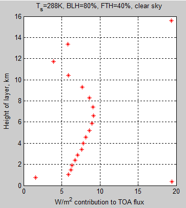
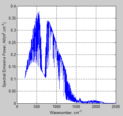
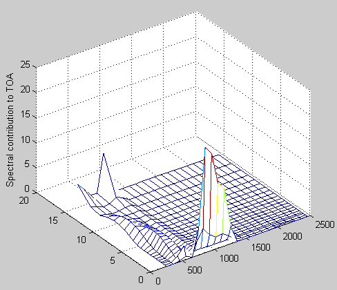
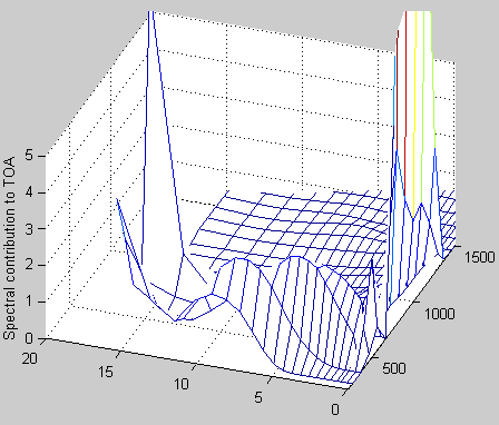
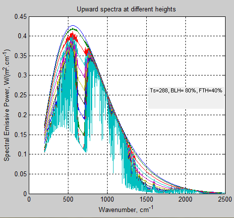
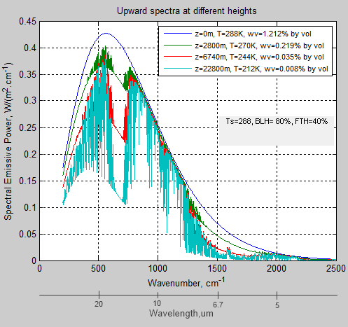
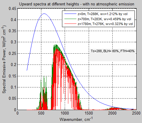
The absorbed solar energy is carried up in the atmosphere by a combination of evapotransporation followed by condensation, thermal convection and radiation (including direct radiation to space, and absorbed and emitted atmospheric radiation). Eventually the conducted, convected, and radiated energy reaches high enough in the atmosphere where it radiates directly to space. This does require absorbing and radiating gases and/or clouds. The sum of all the energy radiated to space from the different altitudes has to equal the absorbed solar energy for the equilibrium case.

The key point is that the outgoing radiation average location is raised significantly above the surface. A single average altitude for outgoing radiation generally is used to replace the outgoing radiation altitude range. The temperature of the atmosphere at this average altitude then is calculated by matching the outgoing radiation to the absorbed solar radiation. The environmental lapse rate, combined with the temperature at the average altitude required to balance incoming and outgoing energy, allows the surface temperature to be then calculated.

The equation for the effect is:

T’ = To -ΓH ….(9)

Where To is the average surface temperature for the non-absorbing atmospheric gases case, with all radiation to space directly from the surface, Γ is the lapse rate (negative as shown), and H is the effective average altitude of outgoing radiation to space. The combined methods that transport energy up so that it radiated to space, are variations of energy transport resistance compared to direct radiation from the surface. In the end, the only factors that raise ground temperature to be higher than the case with no greenhouse gas is the increase in average altitude of outgoing radiation and the lapse rate. That is all there is to the so-called greenhouse effect. If the lapse rate or albedo is changed by addition of specific gases, this is a separate effect, and is not included here.

The case of Venus is a clear example of this effect. The average altitude where radiation to space occurs is about 50 km. The average lapse rate on Venus is about 9 C per km. The surface temperature increase over the case with the same albedo and absorbed insolation but no absorbing or cloud blocking gases, would be about 450 C, so the lapse rate fully explains the increase in temperature.

It is not directly due to the pressure or density alone of the atmosphere, but the resulting increase in altitude of outgoing radiation to space. Changing CO2 concentration (or other absorbing gases) might change the outgoing altitude, but that altitude change would be the only cause of a change in surface temperature, with the lapse rate times the new altitude as the increase in temperature over the case with no absorbing gases.

One point to note is that the net energy transfer (from combined radiation and other transport means) from the surface or from a location in the atmosphere where solar energy was absorbed is always exactly the same whatever the local temperature. For example, the hot surface of Venus radiated up (a very short distance) over 16 kWm-2. However, the total energy transfer up is just the order of absorbed solar energy, or about 17 Wm-2, and some of the energy carried up is by conduction and convection. Thus the net radiation heat transfer is <17 Wm-2, and thus back radiation has to be almost exactly the same as radiation up. The back radiation is not heating the surface; the thermal heat transfer resistance from all causes, including that resulting from back radiation reducing net radiation, results in the excess heating.

In the end, it does not matter what the cause of resistance to heat transfer is. The total energy balance and thermal heat transfer resistance defines the process. For planets with enough atmosphere, the lapse rate defines the lower atmosphere temperature gradient, and if the lapse rate is not changed, the distance the location of outgoing radiation is moved up by addition of absorbing gases determines the increase in temperature effect. It should be clear the back radiation did not do the heating; it is a result of the effect, not the cause.

—— End of section 1 ——

My Response

I agree with Leonard. Now for his rebuttal..

Ok, a few words of clarification. I agree with Leonard about the greenhouse mechanism, the physics and the maths but see a semantic issue about back radiation. It’s always possible it’s a point of substance disguised as a semantic issue but I think that is unlikely.

A large number of people are unhappy about climate science basics but are unencumbered by any knowledge of radiative heat transfer theory as taught in heat transfer textbooks. This group of people claim that back radiation has no effect on the surface temperature. I’ll call them Group Zero. Because of this entertaining and passionate group of people I have spent much time explaining back radiation and physics basics. Perhaps this has led others to the idea that I have a different idea about the mechanism of the inappropriately-named “greenhouse” effect.

Group Zero are saying something completely different from Leonard. Here’s my graphic of Leonard’s explanation from one of his simplified scenarios:

Figure 2 – again

From the maths it is clear that the downward radiation from the shell (shield) is absorbed by the surface and re-emitted. Here the usual graphic presented by the Group Zero position, replete with all necessary equations:

Figure 3 – how can you argue with this?

And here’s an interpretation of a Group Zero concept, pieced together by me from many happy hours of fruitless discussion:

Figure 4 – Group Z?

In this case P, the internal heating, is still a known value. But Y and X are unknown, which is why I have changed them from the solution values shown in figure 2.

Now we have to figure out what they are. Let’s make the assumption that the shell radiates equally inwards and outwards, which is true if it is thin (and so upper and lower surfaces will be at the same temperature) and has the same emissivity both sides. That is why we see the upward flux and the downward flux from the shell both = Y.

Because, according to Group Zero, the downward radiation from a colder atmosphere cannot “have any effect on” the surface, I’m going to assume their same approach to the radiation shield (the “shell”). So the surface only has the energy source P. Group Zero never really explain what happens to Y when it “reaches the ground” but that’s another story. (Although it would be quite interesting to find out along with an equation).

So at the surface, energy in = energy out.

P=X ….(10)

And at the shell, energy in = energy out.

X = 2Y ….(11)

In figure 2, by using real physics we see that the surface emission of radiation by the ball = 2P. This means the surface temperature, T’ = (2P/σ)0.25.

In figure 4, by using invented physics we see that the surface emission of radiation by the ball = P. This means the surface temperature, T'(invented) = (P/σ)0.25.

So the real surface temperature, T’ is 1.19 times larger than T'(invented). Because 20.25 = 1.19.

And back to the important point about the “greenhouse” effect. Because the atmosphere is quite opaque to radiation due to radiatively-active gases like water vapor and CO2 the emission of radiation to space from the climate system is from some altitude. And because temperature reduces with height due to other physics the surface must be warmer than the effective radiating point of the atmosphere. This means the surface temperature of the earth is higher than it would be if there were no radiatively-active gases. (The actual maths of the complete explanation takes up a lot more room than this paragraph). This means I completely agree with Leonard about the “greenhouse” effect.

If back radiation were not absorbed by the surface lots of climate effects would be different because the laws of physics would be different. I’m pretty sure that Leonard completely agrees with me on this.

—— End of section 2 ——

Leonard’s Final Comment

I think we are getting very close to agreement on most of the discussion, but I still sense a bit of disagreement to my basic point. However, this seems to be mainly based on difference in semantics, not the logic of the physics. The frequent use of the statement of heat being transferred from the cold to hot surface (like in back radiation), is the main source of the misuse of a term. Energy can be transferred both ways, but heat transfer has a specific meaning. An example of a version of the second law of thermodynamics, which defines limitations in heat transfer, is from the German scientist Rudolf Clausius, who laid the foundation for the second law of thermodynamics in 1850 by examining the relation between heat transfer and work. His formulation of the second law, which was published in German in 1854, may be stated as: “No process is possible whose sole result is the transfer of heat from a body of lower temperature to a body of higher temperature.”

The specific fact of back radiation and resulting energy transfer does result in the lower surface of the cases with radiation resistance going to a higher temperature. However, this is not due to heat being transferred by back radiation, but by the internal supplied power driving the wall to a higher temperature to transfer the same power. The examples of the solid insulation and opaque gas do exactly the same thing, and back heat transfer or even back energy transport is not the cause of the wall going to the higher temperature for those cases. There is no need to invoke a different effect that heat transfer resistance for the radiation case.

An example can give some insight on how small radiation heat transfer can be even in the presence of huge forward and back radiation effects. For this example we use an example with surface temperature like that found on Venus.

Choose a ball with a small gap with a vacuum, followed by an insulation layer large enough to cause a large temperature variation. The internal surface power to be radiated then conducted out is 17 Wm-2 (similar to absorbed solar surface heating on Venus). The insulation layer is selected thick enough and low enough thermal conductivity so that the bottom of the insulation the wall is 723K (similar to the surface temperature on Venus). The outside insulation surface would only be at 131.6K for this case.

The question is: what is the surface temperature of the ball under the gap?

From my equation (6), the surface of the ball would be 723.2K. The radiation gap caused an increase in surface temperature of 0.2K, which is only 0.033% of the temperature increase. The radiation from the surface of the ball had increased from 17 Wm-2 (for no insulation) to 15,510 Wm-2 due to the combined radiation gap and insulation, and back radiation to the ball is 15,503 Wm-2. This resulted in the net 17 Wm-2 heat transfer. However, the only source of the net energy causing the final wall temperature was the resistance to heat transfer causing the supplied 17 Wm-2 to continually raise the wall temperature until the net out was 17 Wm-2. Nowhere did the back radiation add net energy to the ball wall, even though the back radiation absorbed was huge.

Read Full Post »

« Newer Posts - Older Posts »