In Part Seven we looked at a couple of papers from 1989 and 1994 which attempted to use GCMs to “start an ice age”. The evolution of the “climate science in progress” has been:
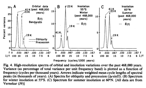
- Finding indications that the timing of ice age inception was linked to redistribution of solar insolation via orbital changes – possibly reduced summer insolation in high latitudes (Hays et al 1976 – discussed in Part Three)
- Using simple energy balance models to demonstrate there was some physics behind the plausible ideas (we saw a subset of the plausible ideas in Part Six – Hypotheses Abound)
- Using a GCM with the starting conditions of around 115,000 years ago to see if “perennial snow cover” could be achieved at high latitudes that weren’t ice covered in the last inter-glacial – i.e., can we start a new ice age?
Why, if an energy balance model can “work”, i.e., produce perennial snow cover to start a new ice age, do we need to use a more complex model? As Rind and his colleagues said in their 1989 paper:
Various energy balance climate models have been used to assess how much cooling would be associated with changed orbital parameters.. With the proper tuning of parameters, some of which is justified on observational grounds, the models can be made to simulate the gross glacial/interglacial climate changes. However, these models do not calculate from first principles all the various influences on surface air temperature noted above, nor do they contain a hydrologic cycle which would allow snow cover to be generated or increase. The actual processes associated with allowing snow cover to remain through the summer will involve complex hydrologic and thermal influences, for which simple models can only provide gross approximations.
[Emphases added – and likewise in all following quotations, bold is emphasis added]. So interestingly, moving to a more complex model with better physics showed that there was a problem with (climate models) starting an ice age. Still, that was early GCMs with much more limited computing power. In this article we will look at the results a decade or so later.
Reviews
We’ll start with a couple of papers that include excellent reviews of “the problem so far”, one in 2002 by Yoshimori and his colleagues and one in 2004 by Vettoretti & Peltier. Yoshimori et al 2002:
One of the fundamental and challenging issues in paleoclimate modelling is the failure to capture the last glacial inception (Rind et al. 1989)..
..Between 118 and 110 kaBP, the sea level records show a rapid drop of 50 – 80 m from the last interglacial, which itself had a sea level only 3 – 5 m higher than today. This sea level lowering, as a reference, is about half of the last glacial maximum. ..As the last glacial inception offers one of few valuable test fields for the validation of climate models, particularly atmospheric general circulation models (AGCMs), many studies regarding this event have been conducted.
Phillipps & Held (1994) and Gallimore & Kutzbach (1995).. conducted a series of sensitivity experiments with respect to orbital parameters by specifying several extreme orbital configurations. These included a case with less obliquity and perihelion during the NH winter, which produces a cooler summer in the NH. Both studies came to a similar conclusion that although a cool summer orbital configuration brings the most favorable conditions for the development of permanent snow and expansion of glaciers, orbital forcing alone cannot account for the permanent snow cover in North America and Europe.
This conclusion was confirmed by Mitchell (1993), Schlesinger & Verbitsky (1996), and Vavrus (1999).. ..Schlesinger & Verbitsky (1996), integrating an ice sheet-asthenosphere model with AGCM output, found that a combination of orbital forcing and greenhouse forcing by reduced CO2 and CH4 was enough to nucleate ice sheets in Europe and North America. However, the simulated global ice volume was only 31% of the estimate derived from proxy records.
..By using a higher resolution model, Dong & Valdes (1995) simulated the growth of perennial snow under combined orbital and CO2 forcing. As well as the resolution of the model, an important difference between their model and others was the use of “envelope orography” [playing around with the height of land].. found that the changes in sea surface temperature due to orbital perturbations played a very important role in initiating the Laurentide and Fennoscandian ice sheets.
And as a note on the last quote, it’s important to understand that these studies were with an Atmospheric GCM, not an Atmospheric Ocean GCM – i.e., a model of the atmosphere with some prescribed sea surface temperatures (these might be from a separate run using a simpler model, or from values determined from proxies). The authors then comment on the potential impact of vegetation:
..The role of the biosphere in glacial inception has been studied by Gallimore & Kutzbach (1996), de Noblet et al. (1996), and Pollard and Thompson (1997).
..Gallimore & Kutzbach integrated an AGCM with a mixed layer ocean model under five different forcings: 1) control; 2) orbital; 3) #2 plus CO2; 4) #3 plus 25% expansion of tundra based on the study of Harrison et al. (1995); and (5) #4 plus further 25% expansion of tundra. The effect of the expansion of tundra through a vegetation-snow masking feedback was approximated by increasing the snow cover fraction. In only the last case was perennial snow cover seen..
..Pollard and Thompson (1997) also conducted an interactive vegetation and AGCM experiment under both orbital and CO2 forcing. They further integrated a dynamic ice-sheet model for 10 ka under the surface mass balance calculated from AGCM output using a multi-layer snow/ice-sheet surface column model on the grid of the dynamical ice-sheet model including the effect of refreezing of rain and meltwater. Although their model predicted the growth of an ice sheet over Baffin Island and the Canadian Archipelago, it also predicted a much faster growth rate in north western Canada and southern Alaska, and no nucleation was seen on Keewatin or Labrador [i.e. the wrong places]. Furthermore, the rate of increase of ice volume over North America was an order of magnitude less than that estimated from proxy records.
They conclude:
It is difficult to synthesise the results of these earlier studies since each model used different parameterisations of unresolved physical processes, resolution, and had different control climates as well as experimental design.
They summarize that results to date indicate that orbital forcing alone nor CO2 alone can explain glacial inception, and the combined effects are not consistent. And the difficulty appears to relate to the resolution of the model or feedback from the biosphere (vegetation).
A couple of years later Vettoretti & Peltier (2004) had a good review at the start of their paper.
Initial attempts to gain deeper understanding of the nature of the glacial–interglacial cycles involved studies based upon the use of simple energy balance models (EBMs), which have been directed towards the simulation of perennial snow cover under the influence of appropriately modified orbital forcing (e.g. Suarez and Held, 1979).
Analyses have since evolved such that the models of the climate system currently employed include explicit coupling of ice sheets to the EBM or to more complete AGCM models of the atmosphere.
The most recently developed models of the complete 100 kyr iceage cycle have evolved to the point where three model components have been interlinked, respectively, an EBM of the atmosphere that includes the influence of ice-albedo feedback including both land ice and sea ice, a model of global glaciology in which ice sheets are forced to grow and decay in response to meteorologically mediated changes in mass balance, and a model of glacial isostatic adjustment, through which process the surface elevation of the ice sheet may be depressed or elevated depending upon whether accumulation or ablation is dominant..
..Such models have also been employed to investigate the key role that variations in atmospheric carbon dioxide play in the 100 kyr cycle, especially in the transition out of the glacial state (Tarasov and Peltier, 1997; Shackleton, 2000). Since such models are rather efficient in terms of the computer resources required to integrate them, they are able to simulate the large number of glacial– interglacial cycles required to understand model sensitivities.
There has also been a movement within the modelling community towards the use of models that are currently referred to as earth models of intermediate complexity (EMICs) which incorporate sub-components that are of reduced levels of sophistication compared to the same components in modern Global ClimateModels (GCMs). These EMICs attempt to include representations of most of the components of the real Earth system including the atmosphere, the oceans, the cryosphere and the biosphere/carbon cycle (e.g. Claussen, 2002). Such models have provided, and will continue to provide, useful insight into long-term climate variability by making it possible to perform a large number of sensitivity studies designed to investigate the role of various feedback mechanisms that result from the interaction between the components that make up the climate system (e.g. Khodri et al., 2003).
Then the authors comment on the same studies and issues covered by Yoshimori et al, and additionally on their own 2003 paper and another study. On their own research:
Vettoretti and Peltier (2003a), more recently, have demonstrated that perennial snow cover is achieved in a recalibrated version of the CCCma AGCM2 solely as a consequence of orbital forcing when the atmospheric CO2 concentration is fixed to the pre-industrial level as constrained by measurements on air bubbles contained in the Vostok ice core (Petit et al., 1999).
This AGCM simulation demonstrated that perennial snow cover develops at high northern latitudes without the necessity of including any feedbacks due to vegetation or other effects. In this work, the process of glacial inception was analysed using three models having three different control climates that were, respectively, the original CCCma cold biased model, a reconfigured model modified so as to be unbiased, and a model that was warm biased with respect to the modern set of observed AMIP2 SSTs.. ..Vettoretti and Peltier (2003b) suggested a number of novel feedback mechanisms to be important for the enhancement of perennial snow cover.
In particular, this work demonstrated that successively colder climates increased moisture transport into glacial inception sensitive regions through increased baroclinic eddy activity at mid- to high latitudes. In order to assess this phenomenon quantitatively, a detailed investigation was conducted of changes in the moisture balance equation under 116 ka BP orbital forcing for the Arctic polar cap. As well as illustrating the action of a ‘‘cyrospheric moisture pump’’, the authors also proposed that the zonal asymmetry of the inception process at high latitudes, which has been inferred on the basis of geological observations, is a consequence of zonally heterogeneous increases and decreases of the northwards transport of heat and moisture.
And they go on to discuss other papers with an emphasis on moisture transport poleward. Now we’ll take a look at some work from that period.
Newer GCM work
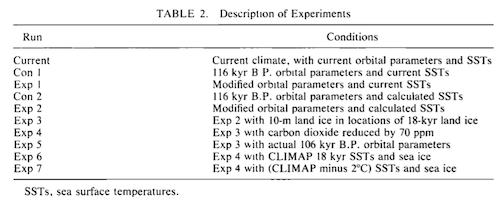
Yoshimori et al 2002
Their models – an AGCM (atmospheric GCM) with 116kyrs orbital conditions and a) present day SSTs b) 116 kyrs SSTs. Then another model run with the above conditions and changed vegetation based on temperature (if the summer temperature is less than -5ºC the vegetation type is changed to tundra). Because running a “fully coupled” GCM (atmosphere and ocean) over a long time period required too much computing resources a compromise approach was used.
The SSTs were calculated using an intermediate complexity model, with a simple atmospheric model and a full ocean model (including sea ice) – and by running the model for 2000 years (oceans have a lot of thermal inertia). The details of this is described in section 2.1 of their paper. The idea is to get some SSTs that are consistent between ocean and atmosphere.
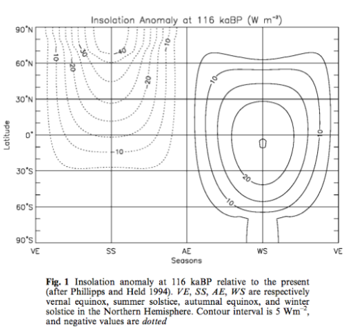
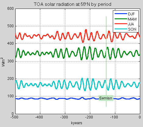
The SSTs are then used as boundary conditions for a “proper” atmospheric GCM run over 10 years – this is described in section 2.2 of their paper. The insolation anomaly, with respect to present day: 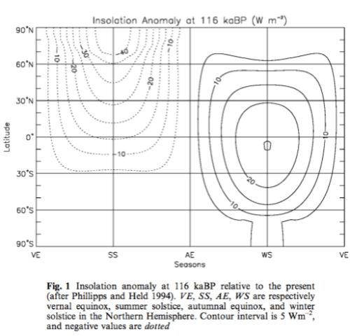
Figure 1
They use 240 ppm CO2 for the 116 kyr condition, as “the lowest probably equivalent CO2 level” (combining radiative forcing of CO2 and CH4). This equates to a reduction of 2.2 W/m² of radiative forcing. The SSTs calculated from the preliminary model are colder globally by 1.1ºC for the 116 kyr condition compared to the present day SST run. This is not due to the insolation anomaly, which just “redistributes” solar energy, it is due to the lower atmospheric CO2 concentration. The 116kyr SST in the northern North Atlantic is about 6ºC colder. This is due to the lower insolation value in summer plus a reduction in the MOC (note 1). The results of their work:
- with modern SSTs, orbital and CO2 values from 116 kyrs – small extension of perennial snow cover
- with calculated 116 kyr SST, orbital and CO2 values – a large extension in perennial snow cover into Northern Alaska, eastern Canada and some other areas
- with vegetation changes (tundra) added – further extension of snow cover north of 60º
They comment (and provide graphs) that increased snow cover is partly from reduced snow melt but also from additional snowfall. This is the case even though colder temperatures generally favor less precipitation.
Contrary to the earlier ice age hypothesis, our results suggest that the capturing of glacial inception at 116kaBP requires the use of “cooler” sea surface conditions than those of the present climate. Also, the large impact of vegetation change on climate suggests that the inclusion of vegetation feedback is important for model validation, at least, in this particular period of Earth history.
What we don’t find out is why their model produces perennial snow cover (even without vegetation changes) where earlier attempts failed. What appears unstated is that although the “orbital hypothesis” is “supported” by the paper, the necessary conditions are colder sea surface temperatures induced by much lower atmospheric CO2. Without the lower CO2 this model cannot start an ice age. And an additional point to note, Vettoretti & Peltier 2004, say this about the above paper:
The meaningfulness of these results, however, remain to be seen as the original CCCma AGCM2 model is cold biased in summer surface temperature at high latitudes and sensitive to the low value of CO2 specified in the simulations.
Vettoretti & Peltier 2003
This is the paper referred to by their 2004 paper.
This simulation demonstrates that entry into glacial conditions at 116 kyr BP requires only the introduction of post-Eemian orbital insolation and standard preindustrial CO2 concentrations
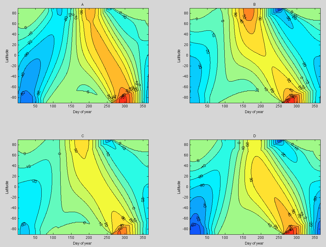
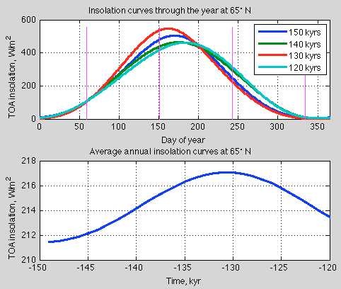
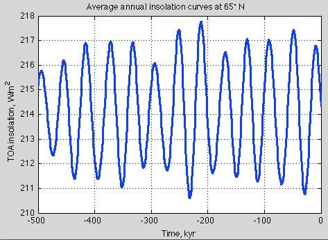
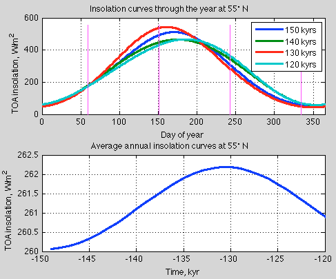
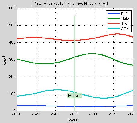
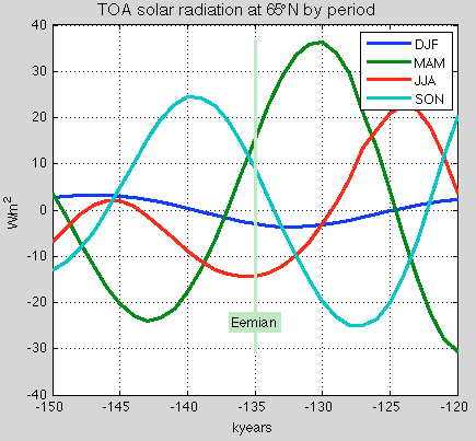
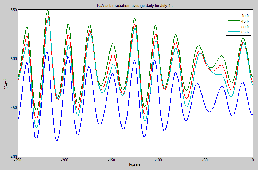
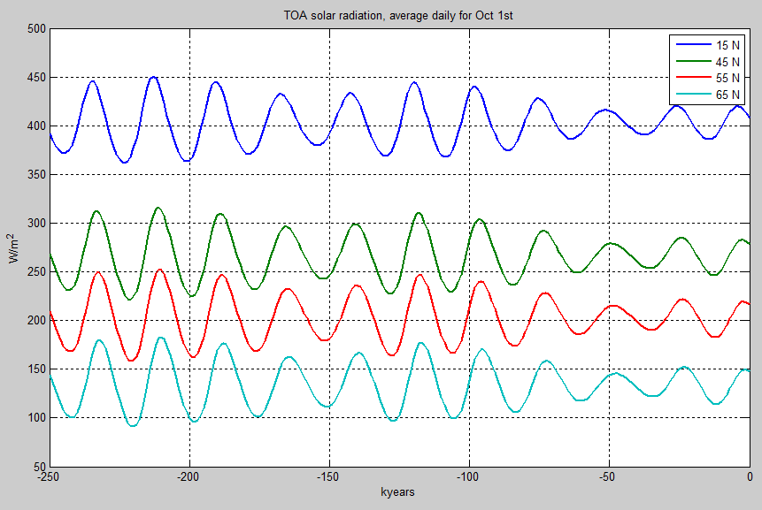
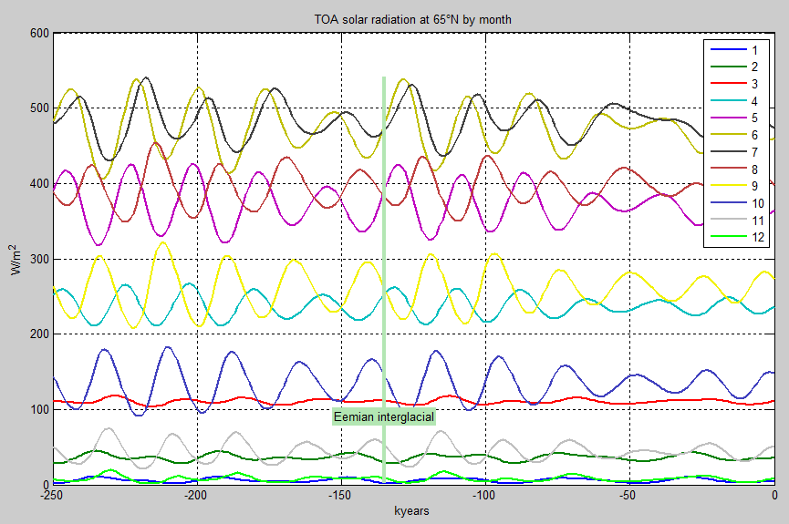
Here are the seasonal and latitudinal variations in solar TOA of 116 kyrs ago vs today:
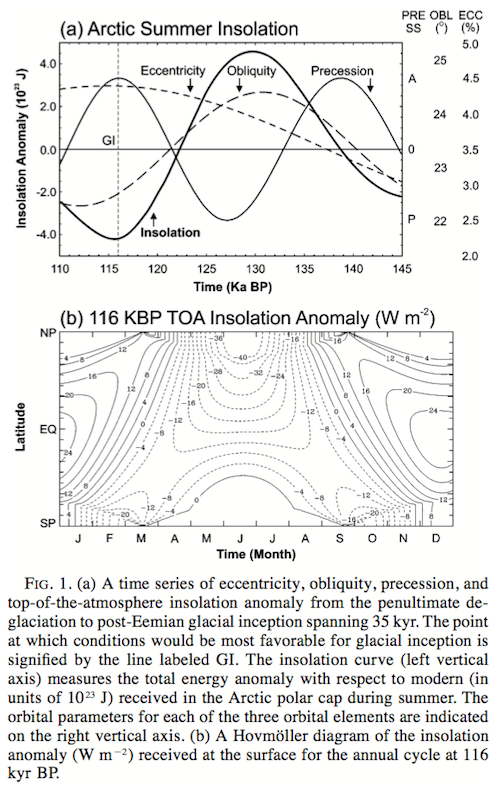
From Vettoretti & Peltier 2003
The essence of their model testing was they took an atmospheric GCM coupled to prescribed SSTs – for three different sets of SSTs – with orbital and GHG conditions from 116 kyrs BP and looked to see if perennial snow cover occurred (and where):
The three 116 kyr BP experiments demonstrated that glacial inception was successfully achieved in two of the three simulations performed with this model.
The warm-biased experiment delivered no perennial snow cover in the Arctic region except over central Greenland.
The cold-biased 116 kyr BP experiment had large portions of the Arctic north of 608N latitude covered in perennial snowfall. Strong regions of accumulation occurred over the Canadian Arctic archipelago and eastern and central Siberia. The accumulation over eastern Siberia appears to be excessive since there is little evidence that eastern Siberia ever entered into a glacial state. The accumulation pattern in this region is likely a result of the excessive precipitation in the modern simulation.
They also comment:
All three simulations are characterized by excessive summer precipitation over the majority of the polar land areas. Likewise, a plot of the annual mean precipitation in this region of the globe (not shown) indicates that the CCCma model is in general wet biased in the Arctic region. It has previously been demonstrated that the CCCma GCMII model also has a hydrological cycle that is more vigorous than is observed (Vettoretti et al. 2000b).
I’m not clear how much the model bias of excessive precipitation also affects their result of snow accumulation in the “right” areas.
In Part II of their paper they dig into the details of the changes in evaporation, precipitation and transport of moisture into the arctic region.
Crucifix & Loutre 2002
This paper (and the following paper) used an EMIC – an intermediate complexity model – which is a trade off model that has courser resolution, simpler parameterization but consequently much faster run time – allowing for lots of different simulations over much longer time periods than can be done with a GCM. The EMICs are also able to have coupled biosphere, ocean, ice sheets and atmosphere – whereas the GCM runs we saw above had only an atmospheric GCM with some method of prescribing sea surface temperatures.
This study addresses the mechanisms of climatic change in the northern high latitudes during the last interglacial (126–115 kyr BP) using the earth system model of intermediate complexity ‘‘MoBidiC’’.
Two series of sensitivity experiments have been performed to assess (a) the respective roles played by different feedbacks represented in the model and (b) the respective impacts of obliquity and precession..
..MoBidiC includes representations for atmosphere dynamics, ocean dynamics, sea ice and terrestrial vegetation. A total of ten transient experiments are presented here..
..The model simulates important environmental changes at northern high latitudes prior the last glacial inception, i.e.: (a) an annual mean cooling of 5 °C, mainly taking place between 122 and 120 kyr BP; (b) a southward shift of the northern treeline by 14° in latitude; (c) accumulation of perennial snow starting at about 122 kyr BP and (d) gradual appearance of perennial sea ice in the Arctic.
..The response of the boreal vegetation is a serious candidate to amplify significantly the orbital forcing and to trigger a glacial inception. The basic concept is that at a large scale, a snow field presents a much higher albedo over grass or tundra (about 0.8) than in forest (about 0.4).
..It must be noted that planetary albedo is also determined by the reflectance of the atmosphere and, in particular, cloud cover. However, clouds being prescribed in MoBidiC, surface albedo is definitely the main driver of planetary albedo changes.
In their summary:
At high latitudes, MoBidiC simulates an annual mean cooling of 5 °C over the continents and a decrease of 0.3 °C in SSTs.
This cooling is mainly related to a decrease in the shortwave balance at the top-of-the atmosphere by 18 W/m², partly compensated for by an increase by 15 W/m² in the atmospheric meridional heat transport divergence.
These changes are primarily induced by the astronomical forcing but are almost quadrupled by sea ice, snow and vegetation albedo feedbacks. The efficiency of these feedbacks is enhanced by the synergies that take place between them. The most critical synergy involves snow and vegetation and leads to settling of perennial snow north of 60°N starting 122 kyr BP. The temperature-albedo feedback is also responsible for an acceleration of the cooling trend between 122 and 120 kyr BP. This acceleration is only simulated north of 60° and is absent at lower latitudes.
See note 2 for details on the model. This model has a cold bias of up to 5°C in the winter high latitudes.
Calov et al 2005
We study the mechanisms of glacial inception by using the Earth system model of intermediate complexity, CLIMBER-2, which encompasses dynamic modules of the atmosphere, ocean, biosphere and ice sheets. Ice-sheet dynamics are described by the three- dimensional polythermal ice-sheet model SICOPOLIS. We have performed transient experiments starting at the Eemian interglacial, at 126 ky BP (126,000 years before present). The model runs for 26 kyr with time-dependent orbital and CO2 forcings.
The model simulates a rapid expansion of the area covered by inland ice in the Northern Hemisphere, predominantly over Northern America, starting at about 117 kyr BP. During the next 7 kyr, the ice volume grows gradually in the model at a rate which corresponds to a change in sea level of 10 m per millennium.
We have shown that the simulated glacial inception represents a bifurcation transition in the climate system from an interglacial to a glacial state caused by the strong snow-albedo feedback. This transition occurs when summer insolation at high latitudes of the Northern Hemisphere drops below a threshold value, which is only slightly lower than modern summer insolation.
By performing long-term equilibrium runs, we find that for the present-day orbital parameters at least two different equilibrium states of the climate system exist—the glacial and the interglacial; however, for the low summer insolation corresponding to 115 kyr BP we find only one, glacial, equilibrium state, while for the high summer insolation corresponding to 126 kyr BP only an interglacial state exists in the model.
We can get some sense of the simplification of the EMIC from the resolution:
The atmosphere, land- surface and terrestrial vegetation models employ the same grid with latitudinal resolution of 10° and longitudinal resolution of approximately 51°
Their ice sheet model has much more detail, with about 500 “cells” of the ice sheet fitting into 1 cell of the land surface model.
They also comment on the general problems (so far) with climate models trying to produce ice ages:
We speculate that the failure of some climate models to successfully simulate a glacial inception is due to their coarse spatial resolution or climate biases, that could shift their threshold values for the summer insolation, corresponding to the transition from interglacial to glacial climate state, beyond the realistic range of orbital parameters.
Another important factor determining the threshold value of the bifurcation transition is the albedo of snow.
In our model, a reduction of averaged snow albedo by only 10% prevents the rapid onset of glaciation on the Northern Hemisphere under any orbital configuration that occurred during the Quaternary. It is worth noting that the albedo of snow is parameterised in a rather crude way in many climate models, and might be underestimated. Moreover, as the albedo of snow strongly depends on temperature, the under-representation of high elevation areas in a coarse- scale climate model may additionally weaken the snow– albedo feedback.
Conclusion
So in this article we have reviewed a few papers from a decade or so ago that have turned the earlier problems (see Part Seven) into apparent (preliminary) successes.
We have seen two papers using models of “intermediate complexity” and coarse spatial resolution that simulated the beginnings of the last ice age. And we have seen two papers which used atmospheric GCMs linked to prescribed ocean conditions that simulated perennial snow cover in critical regions 116 kyrs ago.
Definitely some progress.
But remember the note that the early energy balance models had concluded that perennial snow cover could occur due to the reduction in high latitude summer insolation – support for the “Milankovitch” hypothesis. But then the much improved – but still rudimentary – models of Rind et al 1989 and Phillipps & Held 1994 found that with the better physics and better resolution they were unable to reproduce this case. And many later models likewise.
We’ve yet to review a fully coupled GCM (atmosphere and ocean) attempting to produce the start of an ice age. In the next article we will take a look at a number of very recent papers, including Jochum et al (2012):
So far, however, fully coupled, nonflux-corrected primitive equation general circulation models (GCMs) have failed to reproduce glacial inception, the cooling and increase in snow and ice cover that leads from the warm interglacials to the cold glacial periods..
..The GCMs failure to recreate glacial inception [see Otieno and Bromwich (2009) for a summary], which indicates a failure of either the GCMs or of Milankovitch’s hypothesis. Of course, if the hypothesis would be the culprit, one would have to wonder if climate is sufficiently understood to assemble a GCM in the first place.
We will also see that the strength of feedback mechanisms that contribute to perennial snow cover varies significantly for different papers.
And one of the biggest problems still being run into is the computing power necessary. From Jochum (2012) again:
This experimental setup is not optimal, of course. Ideally one would like to integrate the model from the last interglacial, approximately 126 kya ago, for 10,000 years into the glacial with slowly changing orbital forcing. However, this is not affordable; a 100-yr integration of CCSM on the NCAR supercomputers takes approximately 1 month and a substantial fraction of the climate group’s computing allocation.
More on this fascinating topic very soon.
Articles in the Series
Part One – An introduction
Part Two – Lorenz – one point of view from the exceptional E.N. Lorenz
Part Three – Hays, Imbrie & Shackleton – how everyone got onto the Milankovitch theory
Part Four – Understanding Orbits, Seasons and Stuff – how the wobbles and movements of the earth’s orbit affect incoming solar radiation
Part Five – Obliquity & Precession Changes – and in a bit more detail
Part Six – “Hypotheses Abound” – lots of different theories that confusingly go by the same name
Part Seven – GCM I – early work with climate models to try and get “perennial snow cover” at high latitudes to start an ice age around 116,000 years ago
Part Seven and a Half – Mindmap – my mind map at that time, with many of the papers I have been reviewing and categorizing plus key extracts from those papers
Part Nine – GCM III – very recent work from 2012, a full GCM, with reduced spatial resolution and speeding up external forcings by a factors of 10, modeling the last 120 kyrs
Part Ten – GCM IV – very recent work from 2012, a high resolution GCM called CCSM4, producing glacial inception at 115 kyrs
Pop Quiz: End of An Ice Age – a chance for people to test their ideas about whether solar insolation is the factor that ended the last ice age
Eleven – End of the Last Ice age – latest data showing relationship between Southern Hemisphere temperatures, global temperatures and CO2
Twelve – GCM V – Ice Age Termination – very recent work from He et al 2013, using a high resolution GCM (CCSM3) to analyze the end of the last ice age and the complex link between Antarctic and Greenland
Thirteen – Terminator II – looking at the date of Termination II, the end of the penultimate ice age – and implications for the cause of Termination II
Fourteen – Concepts & HD Data – getting a conceptual feel for the impacts of obliquity and precession, and some ice age datasets in high resolution
Fifteen – Roe vs Huybers – reviewing In Defence of Milankovitch, by Gerard Roe
Sixteen – Roe vs Huybers II – remapping a deep ocean core dataset and updating the previous article
Seventeen – Proxies under Water I – explaining the isotopic proxies and what they actually measure
Eighteen – “Probably Nonlinearity” of Unknown Origin – what is believed and what is put forward as evidence for the theory that ice age terminations were caused by orbital changes
Nineteen – Ice Sheet Models I – looking at the state of ice sheet models
References
On the causes of glacial inception at 116 kaBP, Yoshimori, Reader, Weaver & McFarlane, Climate Dynamics (2002) – paywall paper – free paper
Sensitivity of glacial inception to orbital and greenhouse gas climate forcing, Vettoretti & Peltier, Quaternary Science Reviews (2004) – paywall paper
Post-Eemian glacial inception. Part I: the impact of summer seasonal temperature bias, Vettoretti & Peltier, Journal of Climate (2003) – free paper
Post-Eemian Glacial Inception. Part II: Elements of a Cryospheric Moisture Pump, Vettoretti & Peltier, Journal of Climate (2003)
Transient simulations over the last interglacial period (126–115 kyr BP): feedback and forcing analysis, Crucifix & Loutre 2002, Climate Dynamics (2002) – paywall paper with first 2 pages viewable for free
Transient simulation of the last glacial inception. Part I: glacial inception as a bifurcation in the climate system, Calov, Ganopolski, Claussen, Petoukhov & Greve, Climate Dynamics (2005) – paywall paper with first 2 pages viewable for free
True to Milankovitch: Glacial Inception in the New Community Climate System Model, Jochum et al, Journal of Climate (2012) – free paper
Notes
1. MOC = meridional overturning current. The MOC is the “Atlantic heat conveyor belt” where the cold salty water in the polar region of the Atlantic sinks rapidly and forms a circulation which pulls (warmer) surface equatorial waters towards the poles.
2. Some specifics on MoBidiC from the paper to give some idea of the compromises:
MoBidiC links a zonally averaged atmosphere to a sectorial representation of the surface, i.e. each zonal band (5° in latitude) is divided into different sectors representing the main continents (Eurasia–Africa and America) and oceans (Atlantic, Pacific and Indian). Each continental sector can be partly covered by snow and similarly, each oceanic sector can be partly covered by sea ice (with possibly a covering snow layer). The atmospheric component has been described by Galle ́e et al. (1991), with some improvements given in Crucifix et al. (2001). It is based on a zonally averaged quasi-geostrophic formalism with two layers in the vertical and 5° resolution in latitude. The radiative transfer is computed by dividing the atmosphere into up to 15 layers.
The ocean component is based on the sectorially averaged form of the multi-level, primitive equation ocean model of Bryan (1969). This model is extensively described in Hovine and Fichefet (1994) except for some minor modifications detailed in Crucifix et al. (2001). A simple thermodynamic–dynamic sea-ice component is coupled to the ocean model. It is based on the 0-layer thermodynamic model of Semtner (1976), with modifications introduced by Harvey (1988a, 1992). A one-dimensional meridional advection scheme is used with ice velocities prescribed as in Harvey (1988a). Finally, MoBidiC includes the dynamical vegetation model VE- CODE developed by Brovkin et al. (1997). It is based on a continuous bioclimatic classification which describes vegetation as a composition of simple plant functional types (trees and grass). Equilibrium tree and grass fractions are parameterised as a function of climate expressed as the GDD0 index and annual precipitation. The GDD0 (growing degree days above 0) index is defined as the cumulate sum of the continental temperature for all days during which the mean temperature, expressed in degrees, is positive.
MoBidiC’s simulation of the present-day climate has been discussed at length in (Crucifix et al. 2002). We recall its main features. The seasonal cycle of sea ice is reasonably reproduced with an Arctic sea-ice area ranging from 5 · 106 (summer) to 15 · 106 km2 (winter), which compares favourably with present-day observations (6.2 · 106 to 13.9 · 106 km2, respectively, Gloersen et al. 1992). Nevertheless, sea ice tends to persist too long in spring, and most of its melting occurs between June and August, which is faster than in the observations. In the Atlantic Ocean, North Atlantic Deep Water forms mainly between 45 and 60°N and is exported at a rate of 12.4 Sv to the Southern Ocean. This export rate is compatible with most estimates (e.g. Schmitz 1995). Furthermore, the main water masses of the ocean are well reproduced, with recirculation of Antarctic Bottom Water below the North Atlantic Deep Water and formation of Antarctic Intermediate Water. However no convection occurs in the Atlantic north of 60°N, contrary to the real world. As a consequence, continental high latitudes suffer of a cold bias, up to 5 °C in winter. Finally, the treeline is around about 65°N, which is roughly comparable to zonally averaged observations (e.g. MacDonald et al. 2000) but experiments made with this model to study the Holocene climate revealed its tendency to overestimate the amplitude of the treeline shift in response to the astronomical forcing (Crucifix et al. 2002).
Read Full Post »