The subject of EMICs – Earth Models of Intermediate Complexity – came up in recent comments on Ghosts of Climates Past – Eleven – End of the Last Ice age. I promised to write something about EMICs, in part because of my memory of a more recent paper on EMICs. This article will just be short as I found that I have already covered some of the EMIC ground.
In the previous 19 articles of this series we’ve seen a concise summary (just kidding) of the problems of modeling ice ages. That is, it is hard to model ice ages for at least three reasons:
- knowledge of the past is hard to come by, relying on proxies which have dating uncertainties and multiple variables being expressed in one proxy (so are we measuring temperature, or a combination of temperature and other variables?)
- computing resources make it impossible to run a GCM at current high resolution for the 100,000 years necessary, let alone to run ensembles with varying external forcings and varying parameters (internal physics)
- lack of knowledge of key physics, specifically: ice sheet dynamics with very non-linear behavior; and the relationship between CO2, methane and the ice age cycles
The usual approach using GCMs is to have some combination of lower resolution grids, “faster” time and prescribed ice sheets and greenhouse gases.
These articles cover the subject:
Part Seven – GCM I – early work with climate models to try and get “perennial snow cover” at high latitudes to start an ice age around 116,000 years ago
Part Eight – GCM II – more recent work from the “noughties” – GCM results plus EMIC (earth models of intermediate complexity) again trying to produce perennial snow cover
Part Nine – GCM III – very recent work from 2012, a full GCM, with reduced spatial resolution and speeding up external forcings by a factors of 10, modeling the last 120 kyrs
Part Ten – GCM IV – very recent work from 2012, a high resolution GCM called CCSM4, producing glacial inception at 115 kyrs
One of the the papers I thought about covering in this article (Calov et al 2005) is already briefly covered in Part Eight. I would like to highlight one comment I made in the conclusion of Part Ten:
What the paper [Jochum et al, 2012] also reveals – in conjunction with what we have seen from earlier articles – is that as we move through generations and complexities of models we can get success, then a better model produces failure, then a better model again produces success. Also we noted that whereas the 2003 model (also cold-biased) of Vettoretti & Peltier found perennial snow cover through increased moisture transport into the critical region (which they describe as an “atmospheric–cryospheric feedback mechanism”), this more recent study with a better model found no increase in moisture transport.
So, onto a little more about EMICs.
There are two papers from 2000/2001 describing the CLIMBER-2 model and the results from sensitivity experiments. These are by the same set of authors – Petoukhov et al 2000 & Ganopolski et al 2001 (see references).
Here is the grid:
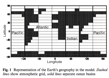
From Petoukhov et al (2000)
The CLIMBER-2 model has a low spatial resolution which only resolves individual continents (subcontinents) and ocean basins (fig 1). Latitudinal resolutions is the same for all modules (10º). In the longitudinal direction the Earth is represented by seven equal sectors (roughly 51º longitude) in the atmosphere and land modules.
The ocean model is a zonally averaged multibasin model, which in longitudinal direction resolves only three ocean basins Atlantic, Indian, Pacific). Each ocean grid cell communicates with either one, two or three atmosphere grid cells, depending on the width of the ocean basin. Very schematic orography and bathymetry are prescribed in the model, to represent the Tibetan plateau, the high Antarctic elevation and the presence of the Greenland-Scotland sill in the Atlantic ocean.
The atmospheric model has a simplified approach, leading to the description 2.5D model. The time step can be relaxed to about 1 day per step. The ocean grid is a little finer in latitude.
On selecting parameters and model “tuning”:
Careful tuning is essential for a new model, as some parameter values are not known a priori and incorrect choices of parameter values compromise the quality and reliability of simulations. At the same time tuning can be abused (getting the right results for the wrong reasons) if there are too many free parameters. To avoid this we adhered to a set of common-sense rules for good tuning practice:
1. Parameters which are known empirically or from theory must not be used for tuning.
2. Where ever possible parametrizations should be tuned separately against observed data, not in the context of the whole model. (Most of the parameters values in Table 1 were obtained in this way and only few of them were determined by tuning the model to the observed climate).
3. Parameters must relate to physical processes, not to specific geographic regions (hidden flux adjustments).
4. The number of tuning parameters must be much smaller than the degrees of freedom predicted by the model. (In our case the predicted degrees of freedom exceed the number of tuning parameters by several orders of magnitude).
To apply the coupled climate model for simulations of climates substantially different from the present, it is crucial to avoid any type of ̄flux adjustment. One of the reasons for the need of ̄flux adjustments in many general circulation models is their high computational cost, which makes optimal tuning difficult. The high speed of CLIMBER-2 allows us to perform many sensitivity experiments required to identify the physical reasons for model problems and the best parameter choices. A physically correct choice of model parameters is fundamentally different from a flux adjustment; only in the former case the surface fluxes are part of the proper feedbacks when the climate changes.
Note that many GCMs back in 2000 did need to use flux adjustment (in Natural Variability and Chaos – Three – Attribution & Fingerprints I commented “..The climate models “drifted”, unless, in deity-like form, you topped up (or took out) heat and momentum from various grid boxes..)
So this all sounds reasonable. Obviously it is a model with less resolution than a GCM, and even the high resolution (by current standards) GCMs need some kind of approach to parameter selection (see Models, On – and Off – the Catwalk – Part Four – Tuning & the Magic Behind the Scenes).
What I remembered about EMICs and suggested in my comment was based on this 2010 paper by Ganopolski, Calov & Claussen:
We will start the discussion of modelling results with a so-called Baseline Experiment (BE). This experiment represents a “suboptimal” subjective tuning of the model parameters to achieve the best agreement between modelling results and palaeoclimate data. Obviously, even with a model of intermediate complexity it is not possible to test all possible combinations of important model parameters which can be considered as free (tunable) parameters.
In fact, the BE was selected from hundred model simulations of the last glacial cycle with different combinations of key model parameters.
Note, that we consider “tunable” parameters only for the ice-sheet model and the SEMI interface, while the utilized climate component of CLIMBER-2 is the same in previous studies, such as those used by C05 [this is Calov et al. (2005)]. In the next section, we will discuss the results of a set of sensitivity experiments, which show that our modelling results are rather sensitive to the choice of the model parameters..
..The ice sheet model and the ice sheet-climate interface contain a number of parameters which are not derived from first principles. They can be considered as “tunable” parameters. As stated above, the BE was subjectively selected from a large suite of experiments as the best fit to empirical data. Below we will discuss results of a number of additional experiments illustrating the sensitivity of simulated glacial cycle to several model parameters. These results show that the model is rather sensitive to a number of poorly constrained parameters and parameterisations, demonstrating the challenges to realistic simulations of glacial cycles with a comprehensive Earth system model.
And in their conclusion:
Our experiments demonstrate that the CLIMBER-2 model with an appropriate choice of model parameters simulates the major aspects of the last glacial cycle under orbital and greenhouse gases forcing rather realistically. In the simulations, the glacial cycle begins with a relatively abrupt lateral expansion of the North American ice sheets and parallel growth of the smaller northern European ice sheets. During the initial phase of the glacial cycle (MIS 5), the ice sheets experience large variations on precessional time scales. Later on, due to a decrease in the magnitude of the precessional cycle and a stabilising effect of low CO2 concentration, the ice sheets remain large and grow consistently before reaching their maximum at around 20 kyr BP..
..From about 19 kyr BP, the ice sheets start to retreat with a maximum rate of sea level rise reaching some 15 m per 1000 years around 15kyrBP. The northern European ice sheets disappeared first, and the North American ice sheets completely disappeared at around 7 kyr BP. Fast sliding processes and the reduction of surface albedo due to deposition of dust play an important role in rapid deglaciation of the NH. Thus our results strongly support the idea about important role of aeolian dust in the termination of glacial cycles proposed earlier by Peltier and Marshall (1995)..
..Results from a set of sensitivity experiments demonstrate high sensitivity of simulated glacial cycle to the choice of some modelling parameters, and thus indicate the challenge to perform realistic simulations of glacial cycles with the computationally expensive models.
My summary – the simplifications of the EMIC combined with the “trying lots of parameters” approach means I have trouble putting much significance on the results.
While the basic setup, as described in the 2000 & 2001 papers seems reasonable, EMICs miss a lot of physics. This is important with something like starting and ending an ice age, where the feedbacks in higher resolution models can significantly reduce the effect seen by lower resolution models. When we run 100’s of simulations with different parameters (relating to the ice sheet) and find the best result I wonder what we’ve actually found.
That doesn’t mean they are of no value. Models help us to understand how the physics of climate actually works, because we can’t do these calculations in our heads. GCMs require too much computing resources to properly study ice ages.
So I look at EMICs as giving some useful insights that need to be validated with more complex models. Or with further study against other observations (what predictions do these parameter selections give us that can be verified?)
I don’t see them as demonstrating that the results “show” we’ve now modeled ice ages. The exact same comment also goes for another 2007 paper which used a GCM coupled to an ice sheet model that we covered in Part Nineteen – Ice Sheet Models I. An update of that paper in 2013 came with a excited Nature press release but to me simply demonstrates that with a few unknown parameters you can get a good result with some specific values of those parameters. This is not at all surprising. Let’s call it a good start.
Perhaps Abe Ouchi et al 2013 was the paper that will be verified as the answer to the question of ice age terminations – the delayed isostatic rebound.
Perhaps Ganopolski, Calov & Claussen 2010 with the interaction of dust on ice sheets will be verified as the answer to that question.
Perhaps neither will be.
Articles in this Series
Part One – An introduction
Part Two – Lorenz – one point of view from the exceptional E.N. Lorenz
Part Three – Hays, Imbrie & Shackleton – how everyone got onto the Milankovitch theory
Part Four – Understanding Orbits, Seasons and Stuff – how the wobbles and movements of the earth’s orbit affect incoming solar radiation
Part Five – Obliquity & Precession Changes – and in a bit more detail
Part Six – “Hypotheses Abound” – lots of different theories that confusingly go by the same name
Part Seven – GCM I – early work with climate models to try and get “perennial snow cover” at high latitudes to start an ice age around 116,000 years ago
Part Seven and a Half – Mindmap – my mind map at that time, with many of the papers I have been reviewing and categorizing plus key extracts from those papers
Part Eight – GCM II – more recent work from the “noughties” – GCM results plus EMIC (earth models of intermediate complexity) again trying to produce perennial snow cover
Part Nine – GCM III – very recent work from 2012, a full GCM, with reduced spatial resolution and speeding up external forcings by a factors of 10, modeling the last 120 kyrs
Part Ten – GCM IV – very recent work from 2012, a high resolution GCM called CCSM4, producing glacial inception at 115 kyrs
Pop Quiz: End of An Ice Age – a chance for people to test their ideas about whether solar insolation is the factor that ended the last ice age
Eleven – End of the Last Ice age – latest data showing relationship between Southern Hemisphere temperatures, global temperatures and CO2
Twelve – GCM V – Ice Age Termination – very recent work from He et al 2013, using a high resolution GCM (CCSM3) to analyze the end of the last ice age and the complex link between Antarctic and Greenland
Thirteen – Terminator II – looking at the date of Termination II, the end of the penultimate ice age – and implications for the cause of Termination II
Fourteen – Concepts & HD Data – getting a conceptual feel for the impacts of obliquity and precession, and some ice age datasets in high resolution
Fifteen – Roe vs Huybers – reviewing In Defence of Milankovitch, by Gerard Roe
Sixteen – Roe vs Huybers II – remapping a deep ocean core dataset and updating the previous article
Seventeen – Proxies under Water I – explaining the isotopic proxies and what they actually measure
Eighteen – “Probably Nonlinearity” of Unknown Origin – what is believed and what is put forward as evidence for the theory that ice age terminations were caused by orbital changes
Nineteen – Ice Sheet Models I – looking at the state of ice sheet models
References
CLIMBER-2: a climate system model of intermediate complexity. Part I: model description and performance for present climate, V Petoukhov, A Ganopolski, V Brovkin, M Claussen, A Eliseev, C Kubatzki & S Rahmstorf, Climate Dynamics (2000)
CLIMBER-2: a climate system model of intermediate complexity. Part II: model sensitivity, A Ganopolski, V Petoukhov, S Rahmstorf, V Brovkin, M Claussen, A Eliseev & C Kubatzki, Climate Dynamics (2001)
Transient simulation of the last glacial inception. Part I: glacial inception as a bifurcation in the climate system, Reinhard Calov, Andrey Ganopolski, Martin Claussen, Vladimir Petoukhov & Ralf Greve, Climate Dynamics (2005)
Simulation of the last glacial cycle with a coupled climate ice-sheet model of intermediate complexity, A. Ganopolski, R. Calov, and M. Claussen, Climate of the Past (2010)


‘… glacial inception as a bifurcation in the climate system…’ Duh.
Where did I read of the inception of the 8.2 ky event as a result of fresh water flooding the Arctic basin? These ‘models’ are special cases of the more common numerical models used. Wave and flood analysis – far simpler in which you may calibrate and then run synthetic data for useful quantification of risk. These climate models seem little more than elaborate hypotheses – and where there are multiple causes involved.
Fresh water inflow, thermohaline feedbacks and runaway ice sheet growth seem a reasonable sequence in the 8.2 ky event but I don’t need a numerical model for that. It suggests a heat related trigger for glacials. Warm evaporation causing excess snow to fall in the Arctic and a large spring thaw. That’s the interesting puzzle – the transition from very warm to very cool very abruptly.
Some models come up with solutions:
“Perhaps Abe Ouchi et al 2013 was the paper that will be verified as the answer to the question of ice age terminations – the delayed isostatic rebound.
Perhaps Ganopolski, Calov & Claussen 2010 with the interaction of dust on ice sheets will be verified as the answer to that question.”
SOD is not so sure: Perhaps neither will be.
I cannot se what the models come up with when it comes to the most important variables. What are the changes in OHC during a glacial cycle. And what is the change in CO2 atmospheric content as a function of temperature during a glacial cycle. I think that models have no credibility if they cannot come up with some answers of those question.
The most logical explanation of the cycles is that oceans build up heat over thousands of years, due to the insulating lid of ice, and that this give a rise in CO2, and a change in currents. That there is a form of global thermostat. From a laymans perspective.
Robert I. Ellison:
“That’s the interesting puzzle – the transition from very warm to very cool very abruptly. ”
Perhaps this abrupt change has been built up over some thousand years. That oceans have lost much heat energy over a long time.
I wonder if there are some proxies that can tell us something of Ocean Heat Content change during the glacial cycles.
I found this paper discussing the Warming of Oceans during glaciation Based on borehole proxies):
Evidence and causes of strong ocean heating during glacial periods.
Sergey A. Zimov, Nikita S. Zimov
North-East Scientific Station, Russian Academy of Sciences
Click to access Zimov_Evidence.pdf
“The uniqueness of the variable Pleistocene climate is likely connected with the fact that very cold and very salty seas and frozen soils, which could accumulate large amounts of carbon, appeared on our planet at the same time. From the analyses presented it follows that during glaciation epochs, haline circulation dominated – the ocean was taking up warm water from the surface and accumulating heat. On land, polar oceans and permafrost were accumulating ice and ocean bottom “ice” (gas clathrates) was melting. Interglacials are epochs when the ocean is dominated by thermo circulation – the ocean absorbs the coldest water and releases its heat. In the ocean bottom, water and methane crystallise while on the land, glaciers and permafrost thaw. Microbes turn into CO2 and CH4, the organic which is accumulated in the permafrost and cold soils Glaciations are periods when the ocean accumulated energy, and interglacials are periods when the ocean quickly released this energy. “
So has the Zimov paper been published anywhere? Probably not, and for good reason. Deep ocean temperatures are pretty much representative of the coldest parts of the surface ocean. (Cold water above warm water is unstable and produces convective mixing that makes the entire column cold. Then the weight of that cold dense column causes the cold water to spread out from the bottom and fill the deep ocean.) So for the deep ocean to reach 23 C, the entire surface ocean would have to be at least that warm, even in the arctic. Maybe during the Cretaceous, but certainly not during glacial periods. And that is what ocean sediments show: https://en.wikipedia.org/wiki/Paleoceanography#Bottom-water_temperature.
There is also the fact that the heat capacity of the ocean is far too small to directly cause glacial periods. It is “only” something like 1000 W-yr/K/m^2. So a 20 C increase in temperature over 100 kyr would amount to about 0.2 W/m^2. That is an order of magnitude smaller than the change in CO2 forcing, which is too small by itself to produce glacial/interglacial transitions.
From what I’ve read, changes in ocean circulation certainly occur and are probably an important part of glacial/interglacial process. As to how that happens, “theories abound”, as SoD titled one post in this series, meaning that no one knows.
It is something called inverse stratification.
“In winter, the exact opposite happens since the lakes are covered with ice. Most of the water under the ice is 39 Fahrenheit; however, there is a thin layer of water under the ice that is colder than 39 and therefore less dense. This thin layer of water floats on top of the lake under the ice throughout the winter, but this stratification is not quite as stable as in the summer because the density difference is much smaller. This concept is called inverse stratification because cooler water is sitting on top of warmer water. Under the ice, the water cannot mix because it is not exposed to wind.”
http://rmbel.info/water-under-the-ice-winter-layers-and-oxygen-levels/
nobodysknowledge,
A layer of ice sitting on top of an ocean that is at 23 C? I don’t think so. And the model you cite only works if the *entire* ocean is covered with ice. Otherwise you will get mixing at least up to the edge of the ice and anyplace that the ice is broken up.
Mike M: I think sediment cores from before ice ages began indicate that the deep ocean was far warmer than today. Of course, we know the Arctic itself was far warmer. The densest water on the planet that was sinking into the deep ocean was warmer than it is today.
nobodysknowledge: Fresh water lakes with ice on top are different from ocean with sea ice. The maximum density of fresh water occurs at 4 degC, but for salt water it is near -2 degC. See Figure 2 of:
http://www.nature.com/scitable/knowledge/library/key-physical-variables-in-the-ocean-temperature-102805293
To my surprise, I found that fresh water of 0 degC has the same density as seawater at 76 degC.
So, in theory we could have an multiyear ice over ocean (ice without any salinity) with some meltwater underneath, stratified over seawater so hot as 70 degC. Conduction would of course destratify it very fast. But an interesting question is how great difference in temperature can it be between fresh meltwater and deeper seawater, and keep stability at the same time.
https://nsidc.org/cryosphere/seaice/environment/global_climate.html
About heat exchange and the insulating effect of ice: “During winter, the Arctic’s atmosphere is very cold. In comparison, the ocean is much warmer. The sea ice cover separates the two, preventing heat in the ocean from warming the overlying atmosphere. This insulating effect is another way that sea ice helps to keep the Arctic cold. But heat can escape rather efficiently from areas of thin ice and especially from leads and polynyas, small openings in the ice cover. Roughly half of the total exchange of heat between the Arctic Ocean and the atmosphere occurs through openings in the ice. With more leads and polynyas, or thinner ice, the sea ice cannot efficiently insulate the ocean from the atmosphere. The Arctic atmosphere then warms, which, in turn influences the global circulation of the atmosphere.”
Mike M:
“A layer of ice sitting on top of an ocean that is at 23 C? I don’t think so.”
I think you are right in this. But an inverse stratification model could still work.
Some scientists have taken the change in deep ocean temperatures and the accumulation of energy serious.
Abrupt pre-Bølling–Allerød warming and circulation changes in the deep ocean
Nivedita Thiagarajan, Adam V. Subhas, John R. Southon, John M. Eiler & Jess F. Adkins
.
“Several large and rapid changes in atmospheric temperature and the partial pressure of carbon dioxide in the atmosphere1—probably linked to changes in deep ocean circulation2—occurred during the last deglaciation. The abrupt temperature rise in the Northern Hemisphere and the restart of the Atlantic meridional overturning circulation at the start of the Bølling–Allerød interstadial, 14,700 years ago, are among the most dramatic deglacial events3, but their underlying physical causes are not known. Here we show that the release of heat from warm waters in the deep North Atlantic Ocean probably triggered the Bølling–Allerød warming and reinvigoration of the Atlantic meridional overturning circulation.”
http://www.nature.com/nature/journal/v511/n7507/full/nature13472.html
So. What do CLIMBER-2 tell us about this?
It has been a while since my last visit. Nothing on this thread makes sense.
I will check again in2017.
gallopingcamel.
Here is something more that make no sense to you about warm ocean under cold water.
“The build-up and subsequent release of warm, stagnant water from the deep Arctic Ocean and Nordic Seas played a role in ending the last Ice Age within the Arctic region, according to new research led by a UCL scientist.
The study, published today in Science, examined how the circulation of the ocean north of Iceland – the combined Arctic Ocean and Nordic Seas, called the Arctic Mediterranean – changed since the end of the last Ice Age (~20,000-30,000 years ago).
Today, the ocean is cooled by the atmosphere during winter, producing large volumes of dense water that sink and flush through the deep Arctic Mediterranean. However, in contrast to the vigorous circulation of today, the research found that during the last Ice Age, the deep Arctic Mediterranean became like a giant stagnant pond, with deep waters not being replenished for up to 10,000 years.
This is thought to have been caused by the thick and extensive layer of sea ice and fresh water that covered much of the Arctic Mediterranean during the Ice Age, preventing the atmosphere from cooling and densifying the underlying ocean.
Dr David Thornalley (UCL Geography) said: “As well as being stagnant, these deep waters were also warm. Sitting around at the bottom of the ocean, they slowly accumulated geothermal heat from the seafloor, until a critical point was reached when the ocean became unstable.
“Suddenly, the heat previously stored in the deep Arctic Mediterranean was released to the upper ocean. The timing of this event coincides with the occurrence of evidence for a massive release of meltwater into the Nordic Seas. We hypothesize that this input of melt water was caused by the release of deep ocean heat, which melted icebergs, sea-ice and surrounding marine-terminating ice sheets.””
From. http://phys.org/news/2015-08-stagnant-deep-sea-ice-age.html
And recent studies of stratification under ice:
4.3. Amundsen Sea: water stratification under fast ice
“The water stratification under fast ice is clearly visible
(Fig. 7a), with the colder water found on the top of the
300 m column. The stratification of salinity is not so clear,
although less saline water was mainly in the top 200 m”
Ocean heat flux under Antarctic sea ice in the Bellingshausen and
Amundsen Seas: two case studies
Stephen F. ACKLEY, Hongjie XIE, Elizabeth A. TICHENOR
Click to access a69a890.pdf
So, CLIMBER-2. You play the aeolian dust parameter card that triumph all ocean warming?
nobodysknowledge,
The Thornalley et al. paper looks interesting, although it also looks like it will take some deciphering. From a quick look at the abstract and figures, it looks like “warm” means roughly 1 C, compared to the modern deep Arctic value of -1.5 C.
I wonder if this will appear as a reply to your post or as a new thread. Dang those scripts.
Mike
You may be right that stratification doesn`t give that much waming in deep high latitude oceans. Still it can be storage of a great amount of energy.
SoD post: ghosts-of-climates-past-part-six-hypotheses-abound
He put foreward two papers with different explanations, that i find interesting.
Self-Oscillations of the Climate System
Broecker & Denton (1990):
We propose that Quaternary glacial cycles were dominated by abrupt reorganizations of the ocean-atmosphere system driven by orbitally induced changes in fresh water transports which impact salt structure in the sea. These reorganizations mark switches between stable modes of operation of the ocean-atmosphere system. Although we think that glacial cycles were driven by orbital change, we see no basis for rejecting the possibility that the mode changes are part of a self-sustained internal oscillation that would operate even in the absence of changes in the Earth’s orbital parameters. If so, as pointed out by Saltzman et al. (1984), orbital cycles can merely modulate and pace a self-oscillating climate system..
Temperature Gradient between Low & High Latitude
George Kukla, Clement, Cane, Gavin & Zebiak (2002):
..At first glance the implications of our results appear to be counterintuitive, indicating that the early buildup of glacier ice was associated not with the cooling, but with a relative warming of tropical oceans. Recent analogs suggest that it might even have been accompanied by a temporary increase of globally averaged annual mean temperature. If correct, the main trigger of glaciations would not be the expansion of snow fields in subpolar belts, but rather the increase in temperature gradient between the low and the high latitudes.
I would think that most of the global warming prior to deglaciation show up in the temperature gradient between low and high latitude, and that it slowly reach higher latitudes. Perhaps together with goethermal heat. The icecap will just help energy accumulation by stopping evaporation and convection/conduction from huge areas of the ocean.
SoD,
“Perhaps Abe Ouchi et al 2013 was the paper that will be verified as the answer to the question of ice age terminations – the delayed isostatic rebound.”
That paper sure gets my vote as the most likely explanation for the rather odd timing of ice ages. There is one other thought I have about ice ages: I have read that the tropics were likely not all that much cooler, even though the temperatures over the ice sheets were certainly much colder. Seems to me the drop in sea level from ice accumulation (~120 meters?) means that everywhere except over the ice sheets the atmosphere was thicker and so presented a somewhat greater resistance to heat loss. If you take the average lapse rate value at 6.5C/Km, that 120 meters of extra air over the rest of the Earth could be expected to raise local surface temperature by about 0.78C.
You’re kidding, right?
Do you want me to calculate exactly how much extra air there would need to be added to the atmosphere for your calculation to be correct?
DeWitt,
Not kidding at all. It’s just conservation of mass. The amount of air is the same. But the effective elevation, and atmospheric pressure at the local surface, at different geographical locations changes. If there is less total air above multi-km high ice sheets, then there is necessarily more above the oceans that are 120 meters lower than today. Heck, the surface elevation of Greenland’s ice sheet today is what ensures the ice sheet surface is almost always below 0C.
I am pretty sure that Steve is right. For a given greenhouse gas concentration, the emission altitude stays at the same place, relative to the center of the earth, for both glacial and interglacial conditions. That is in the upper troposphere, far above any topography. So during glacial times the distance from the surface to the emission altitude is less over the ice caps and more over the oceans. So for a given lapse rate, the ocean surface will be warmer for glacial conditions.
But the might be somewhat less than Steve calculates, since the depression of the crust under the ice should push it up under the oceans, partially restoring sea level.
Mike M,
Yes the crustal accommodation is important and reduces the change in atmospheric density somewhat… but it is delayed by thousands of years. As the weight of the accumulating ice gradually depresses the crust, at some point the altitude of the ice sheet begins to decline, and so becomes relatively warmer, maybe enough to precipitate melting. It’s all tied together. That is why the delayed crustal response makes sense to me.
The center of Greenland is below sea level. The usual map of Antarctica shows what the continent would look like after glacial isostatic rebound, not the edge of the land at current sea level. I like to speculate wildly what Greenland would look like if ice continued to accumulate and the island continued to subside until the whole area was below sea level – and the ice floated away? OK, with 90% of the ice below water level and buoyancy reducing the weight of the ice driving subsistence, it will never float away. But it will melt faster. Do continental glaciers grow until subsidence makes them vulnerable to termination? After enough cycles, could subsidence have slowed enough to produce a shift from vulnerability every 41,000 years or vulnerability every 100,000 years? /wild speculation
SteveF,
Getting old. The total volume of water remains the same to a first order, it just moves. Actually, the ice volume is probably greater than the volume of water from which it came.
Frank,
I think that the heat leak that started when Antarctica separated from South America and was aggravated when the Isthmus of Panama closed was continuing. That’s the root cause of the increase in cycle length.
So we’re saving the planet from an icy tomb by burning fossil fuels. /sarc
DeWitt,
Yes the ~9% expansion of ice versus water exaggerates the effect, but as MikeM notes, crustal accommodation removes more than that much of the effect at the surface of the ice sheet, at least if given enough time. But crustal accommodation itself leads to localized surface uplift in regions adjacent to the ice sheet. If those adjacent regions are dry land, then they will also be a bit cooler than they would otherwise have been. In any case, the tendency ought to be for the altitude of the surfaces of large ice sheets to ‘lock in’ very low local surface temperatures, helping to stabilize the ice sheet against melting for long periods, in spite of increased summertime insolation from orbital changes.
I am not so impressed by Abe Ouchi et al 2013. The 100 ky cycle is not one puzzle, but two: the presence of the cycle in the late Pleistocene and its absence in the early Pleistocene. So a model can be built that explains one but not the other. Big deal. Unless both are explained, neither is explained.
I am not saying that there is nothing of value in Abe Ouchi. It may well be a step in the right direction. But it is not there yet.
The geography changed somewhat, and it is likely CO2, N2O and methane were higher in the pre-glacial period and the short cycle period. The shorter cycles in the earlier record actually make more sense (in terms of orbital forcing) than more recent (longer) cycles. The earlier cycles were also (apparently) more shallow. I don’t think the change from shorter to longer cycles conflicts with having delayed crustal rebound contribute to the pace of more recent longer cycles.
SOD has shown there is something big we don’t understand about terminations. Whatever that may be, it may also be the cause of the change in cycle length. If subsidence is an important factor in triggering terminations, perhaps ten of so short cycles cooled and stiffened the upper mantle, perhaps through an increase in volcanic eruption or simple mixing. But that is still wild speculation.
https://www.sciencedaily.com/releases/2016/01/160104163203.htm?CFID=6583b8b8-c415-46b5-96c1-e03583989390&CFTOKEN=0
A new study reconstructing conditions at the end of the last ice age suggests that as the Antarctic sea ice melted, massive amounts of carbon dioxide that had been trapped in the ocean were released into the atmosphere.
A new study reconstructing conditions at the end of the last ice age suggests that as the Antarctic sea ice melted, massive amounts of carbon dioxide that had been trapped in the ocean were released into the atmosphere.
“Before this study there were these two observations, the first was that glacial deep water was really salty and dense, and the second that it also contained a lot of CO2, and the community put two and two together and said these two observations must be linked,” said Roberts. “But it was only through doing our study, and looking at the change in both density and CO2 across the deglaciation, that we found they actually weren’t linked. This surprised us all.”
Through examination of the shells, the researchers found that changes in CO2 and density are not nearly as tightly linked as previously thought, suggesting something else must be causing CO2 to be released from the ocean.
Like a bottle of wine with a cork, sea ice can prevent CO2-rich water from releasing its CO2 to the atmosphere. The Southern Ocean is a key area of exchange of CO2 between the ocean and atmosphere. The expansion of sea ice during the last ice age acted as a ‘lid’ on the Southern Ocean, preventing CO2 from escaping. The researchers suggest that the retreat of this sea ice lid at the end of the last ice age uncorked this vintage CO2, resulting in an increase in carbon dioxide in the atmosphere.
Jenny Roberts, Julia Gottschalk, Luke C. Skinner, Victoria L. Peck, Sev Kender, Henry Elderfield, Claire Waelbroeck, Natalia Vázquez Riveiros, David A. Hodell. Evolution of South Atlantic density and chemical stratification across the last deglaciation. Proceedings of the National Academy of Sciences, 2016; 201511252 DOI: 10.1073/pnas.1511252113
It is like a bit of the story is not told. CO2 is released from the ocean 5000 years earlier than it is released from deep dense layers. Do this mean that upper layers have stored a lot of CO2, which was released when the ice disappeared. Could the explanation be that the upper layers were colder, and that the water was heated by warm currents, melting the ice, and releasing CO2? And that deeper water was warmer so it could not contain so huge amounts of CO2? It is nothing about water temperatures in the summary.
So, CLIMBER-2. What can you tell us about this?
No. When sea water freezes, much of the salt is excluded. That makes the layer next to the ice more saline and denser, not less. That, of course, causes convection with the colder and denser water sinking to the bottom. That continues until the ice is thick enough so that heat transfer to space from the ~-30°C surface balances the conduction of heat through the ice from the just above freezing water directly below the ice.
What warm currents? What is the heat source?
What warm currents? What is the heat source?
Let me repeat what I wrote earlier: I would think that most of the global warming prior to deglaciation show up in the temperature gradient between low and high latitude, and that it slowly reach higher latitudes. Perhaps together with goethermal heat. The icecap will just help energy accumulation by stopping evaporation and convection/conduction from huge areas of the ocean.
SoD: ghosts-of-climates-past-part-six-hypotheses-abound
Temperature Gradient between Low & High Latitude
George Kukla, Clement, Cane, Gavin & Zebiak (2002):
“..At first glance the implications of our results appear to be counterintuitive, indicating that the early buildup of glacier ice was associated not with the cooling, but with a relative warming of tropical oceans.”
So one theory would be that tropical oceans take up a lot of heat, while ocean currents over higher latitudes fade out. This would build up warm currents at lower latitudes. Combined with ocean temperature and salinity stratification at higher latitudes there cuold be a homeostatic stability for a many thousand years, which at some time would break down.
DeWitt Payne
I think it could be better explanations than the dust of models. even if it is speculations.
The latest news about currents during ice age:
” During the coldest periods of the last ice age the Nordic seas were covered with a permanent layer of sea ice. The pump stopped transporting the heat northward. The heat accumulated in the southern oceans. However, the warming was not restricted to the south.
” Our results show that it continued all the way to Iceland. The warming was slow and gradual, and happened simultaneously in both hemispheres. Little by little the warm Atlantic water penetrated into the Nordic sea underneath the ice cover. It melted the ice from below. Once the ice was gone, the pump started up again, bringing additional warm water into the Nordic seas. And we got a warmer period for 50 years. ” says Rasmussen.
Large ice sheets continued however, to cover the continents around the Nordic seas. In contact with the warm ocean water they started calving. This delivered icebergs and fresh water into the sea and caused a cooling down of the surface water. The seas were again frozen. And the pump slowed down.
The warm ocean blob of the ice ages rewrites the understanding of the ocean circulation systems, and how they affected the extreme climate changes of the past. The seesaw was actually more of a ‘push and pull’ system.
“There are no symmetrical processes in the north and the south — the climate changes were principally governed by simultaneous warming and the constant closing and re-opening of the sink pump in the Nordic seas” says Tine Rasmussen”
Tine L. Rasmussen, Erik Thomsen, Matthias Moros. North Atlantic warming during Dansgaard-Oeschger events synchronous with Antarctic warming and out-of-phase with Greenland climate. Scientific Reports, 2016; 6: 20535 DOI: 10.1038/srep20535
https://www.sciencedaily.com/releases/2016/02/160219134816.htm
So, what are models telling us of change in ocean sink pump? (Which somebody more correctly named ocean waterfall)
Do these models account for isostatic balance? A couple of years ago I did a calculation using a yellow sticky and concluded the ice loads must be causing large vertical movements, which in turn can move the snow line back and forth.
I also noticed the sea level drop (increase) exposed (covered) a lot of land in some areas, and this changes albedo. Does this effect get included? It could be very subtle on a worldwide basis but it could have a very large impact on small sectors.
Now THIS is climate modelling. “Having numerically calculated the solar activity variations, he explaines and predicts the derived climate variability. Most of modern global warming is the result of solar activity variations.”
SOD: Nature has a new paper (paywalled) about glacial terminations. Nature 534, 640–646 (30 June 2016). Can’t tell if this paper addresses any of the mysteries about terminations and installations.
http://www.nature.com/nature/journal/v534/n7609/full/nature18591.html?WT.ec_id=NATURE-20160630&spMailingID=51721378&spUserID=NTYwMTQ5NDQxOTgS1&spJobID=944211569&spReportId=OTQ0MjExNTY5S0
Oxygen isotope records from Chinese caves characterize changes in both the Asian monsoon and global climate. Here, using our new speleothem data, we extend the Chinese record to cover the full uranium/thorium dating range, that is, the past 640,000 years. The record’s length and temporal precision allow us to test the idea that insolation changes caused by the Earth’s precession drove the terminations of each of the last seven ice ages as well as the millennia-long intervals of reduced monsoon rainfall associated with each of the terminations. On the basis of our record’s timing, the terminations are separated by four or five precession cycles, supporting the idea that the ‘100,000-year’ ice age cycle is an average of discrete numbers of precession cycles. Furthermore, the suborbital component of monsoon rainfall variability exhibits power in both the precession and obliquity bands, and is nearly in anti-phase with summer boreal insolation. These observations indicate that insolation, in part, sets the pace of the occurrence of millennial-scale events, including those associated with terminations and ‘unfinished terminations’.
Hello, are you finished posting to the blog (hopefully not)?
PA32R,
Thankyou.
Let’s hope. Been super-busy with company startup, travel, etc.
Also, lots of unanswered questions, that get increasingly difficult to answer. And even to articulate.
I did think about writing an article with the list of my current difficult to answer questions.
Many people writing opinions in their blogs, but what value are opinions?
Thanks for the answer and best of luck with the startup. Your blog is, to the best of my knowledge, absolutely unique in the space of the nexus of climate, energy, and environment. Only a fool (I’m looking at you Bryan) could fail to learn from it and I strongly suspect that you have learned much yourself from publishing not only the posts but addressing the comments. It’s a hugely valuable contribution and the quantity of comments is indicative of that value. Of course, it’s also true that one could make the case of “so what?” but I choose to be more optimistic than that.
SoD says
“Many people writing opinions in their blogs, but what value are opinions?”
PA32R (@PA32R) says
” Only a fool (I’m looking at you Bryan)”
As the man with the wooden leg says…..
Its just a matter of a pinion!
Nobody considers whether the ozone depletion since 1950 is the cause of warmer temperatures.
I’m reasonably sure stratospheric ozone is included in the radiation transfer code in the climate models. The place to start looking is the IPCC Assessment reports. My best guess would be that it does contribute, but it’s not much compared to CO2 and the other ghg’s.
https://www.ipcc.ch/publications_and_data/ar4/wg1/en/ch7s7-4-6.html
Tim: You can address this question yourself by using the online MODTRAN program at: http://climatemodels.uchicago.edu/modtran/modtran.html
Using the US Standard Atmosphere, a uniform 10, 50 or 100% reduction in stratospheric ozone increases – not decreases – TOA OLR by 0.2, 1.6 or 5.4 W/m2. Therefore stratospheric ozone depletion cools the planet, not warms it. Over most of the planet ozone depletion has been well below 10%, though it reaches 50% over Antarctica for a few months in the spring.
Radiative forcing (the instantaneous change) is only part of the story. As the stratosphere cools, the increase in OLR will decrease. MODTRAN doesn’t take stratospheric temperature change into account, but the IPCC’s definition of radiative forcing does. And we need to consider the effect on incoming SWR. Less ozone means somewhat more heat is deposited at the surface rather than the stratosphere.
This figure from AR4 places the [un]importance of past changes in stratospheric ozone in perspective.
https://en.wikipedia.org/wiki/File:Radiative-forcings.svg
Thinking about Tim’s question reminded me about the importance of altitude/temperature to radiative forcing. Suppose the ozone layer were at 50 km, where the temperature 260-270 K; instead of 20-30 km, where the temperature is 210-230. The increased altitude would increase its ability to radiatively cool to space, but not change its ability to absorption.
What if we could geo-engineer the presence of a GHG layer at 50 km where it is relatively warm? For example, we could transport CO2 there. Most outgoing radiation at wavelengths emitted by CO2 comes from the tropopause, where it is far colder. The would be an “inverse-GHE” at this altitude. Of course, it would be hard to keep CO2 localized there with the Brewer-Dobson circulation
If we dream bigger, we could put the CO2 (or water vapor) above the turbopause in the thermosphere.
Frank,
You couldn’t put much of any gas in the thermosphere. The pressure is too low. It would all fall back down to a lower altitude. The stratospheric ozone layer is where it is because that’s where the partial pressure of oxygen becomes sufficient to form enough ozone to absorb significant amounts of UV radiation.
If I have the right info, at 120 km (0.00003 mb) the temperature is 400 K (assuming that the word temperature has a meaning at that altitude). The ozone layer at 25 km (30 mb) has only 10 ppm of ozone, but that is enough to decrease OLR by 5.4 W/m2. Let’s call that 300 mb-ppm of ozone. OLR decreases only because upwelling radiation at this wavelength originates at the surface, where it is 290 K and is absorbed by ozone at 210-230 K. If CO2 or H2O interacted with OLR as strongly as O3, pure CO2 or H2O (1,000,000 ppm) would have a concentration of 30 mb-ppm. Since you have a much larger temperature differential, pure CO2 or water would be more than enough.
Unfortunately, LTE doesn’t exist at this altitude and emission depends on temperature and the local radiation field. I’m not sure a thermosphere with mostly CO2 would be as hot as our planet’s. Perhaps we know from Venus.
Frank,
The thermosphere is also where the pressure vs. altitude profile depends on molecular or atomic weight because, being above the turbopause, the atmosphere cannot be considered well mixed.