I generally try and avoid the media as much as possible (although the 2016 Circus did suck me in) but it’s still impossible to miss claims like the following:
Climate change is already causing worsening storms, floods and droughts
Before looking at predictions for the future I thought it was worth reviewing this claim, seeing as it is so prevalent and is presented as being the current consensus of climate science.
Droughts
SREX 2012, p. 171:
There is medium confidence that since the 1950s some regions of the world have experienced more intense and longer droughts (e.g., southern Europe, west Africa) but also opposite trends exist in other regions (e.g., central North America, northwestern Australia).
The report cites Sheffield and Wood 2008 who show graphs on a variety of drought metrics from around the world over the last 50 years – click to enlarge:
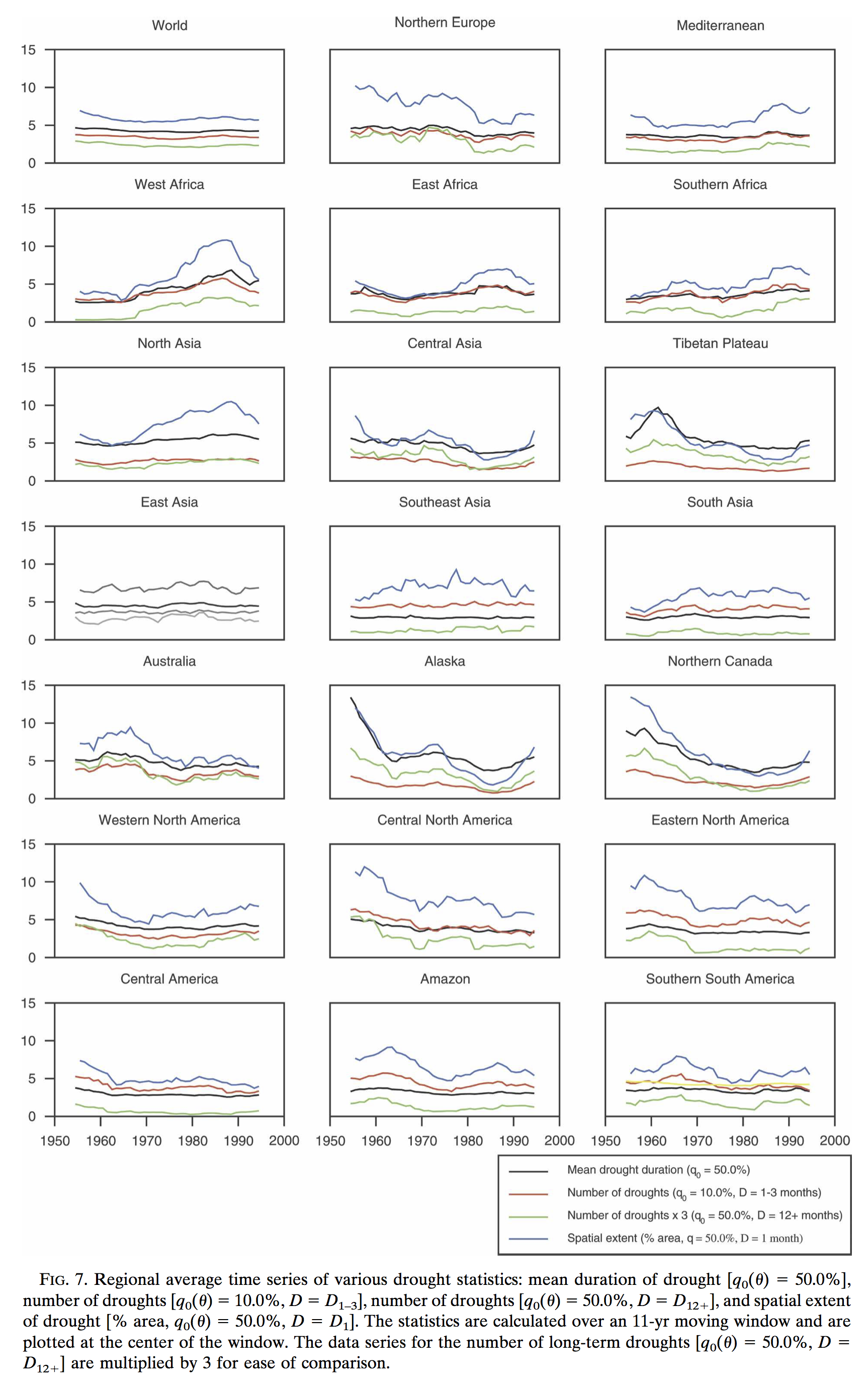
From Sheffield & Wood 2008
Figure 1 – Click to enlarge
The results above were calculated from models based on available meteorological data. According to their analysis some places have experienced more droughts, and other places less droughts. Because they are based on models we can expect that alternative researchers may produce different results.
AR5, published a year after SREX, says, chapter 2, p. 214-215:
Because drought is a complex variable and can at best be incompletely represented by commonly used drought indices, discrepancies in the interpretation of changes can result. For example, Sheffield and Wood (2008) found decreasing trends in the duration, intensity and severity of drought globally. Conversely, Dai (2011a,b) found a general global increase in drought, although with substantial regional variation and individual events dominating trend signatures in some regions (e.g., the 1970s prolonged Sahel drought and the 1930s drought in the USA and Canadian Prairies). Studies subsequent to these continue to provide somewhat different conclusions on trends in global droughts and/ or dryness since the middle of the 20th century (Sheffield et al., 2012; Dai, 2013; Donat et al., 2013c; van der Schrier et al., 2013)..
..In summary, the current assessment concludes that there is not enough evidence at present to suggest more than low confidence in a global-scale observed trend in drought or dryness (lack of rainfall) since the middle of the 20th century, owing to lack of direct observations, geographical inconsistencies in the trends, and dependencies of inferred trends on the index choice.
Based on updated studies, AR4 conclusions regarding global increasing trends in drought since the 1970s were probably overstated.
The paper by Dai is Drought under global warming: a review, A Dai, Climate Change (2011) – for some reason I am unable to access it.
A later paper in Nature, Trenberth et al 2013 (including both Sheffield and Dai as co-authors) said:
Two recent papers looked at the question of whether large-scale drought has been increasing under climate change. A study in Nature by Sheffield et al entitled ‘Little change in global drought over the past 60 years’ was published at almost the same time that ‘Increasing drought under global warming in observations and models’ by Dai appeared in Nature Climate Change (published online in August 2012). How can two research groups arrive at such seemingly contradictory conclusions?
Another later paper on droughts, Orlowski & Seneviratne 2013, likewise shows overwhelming evidence of more droughts – click to enlarge:
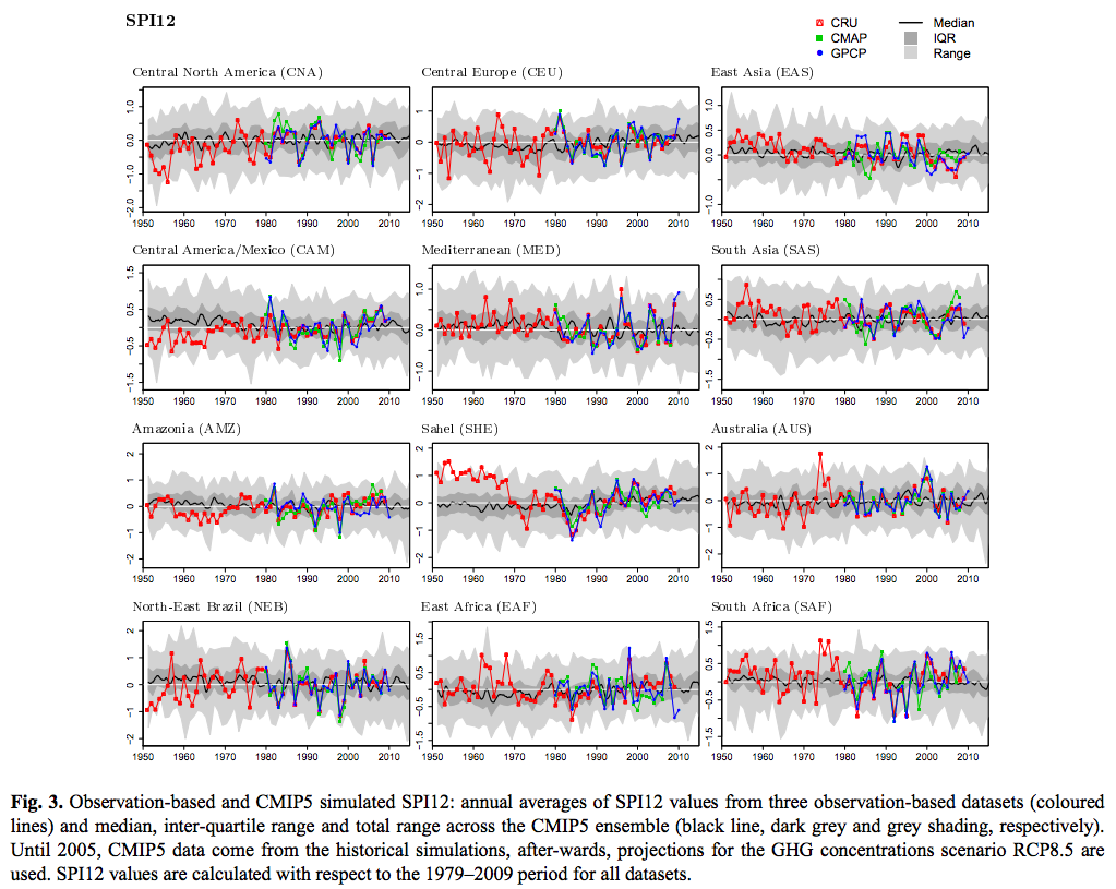
From Orlowsky & Seneviratne 2013
Figure 2 – Click to enlarge
Floods
SREX 2012, p. 177:
Overall, there is low confidence (due to limited evidence) that anthropogenic climate change has affected the magnitude and frequency of floods, though it has detectably influenced several components of the hydrological cycle, such as precipitation and snowmelt, that may impact flood trends. The assessment of causes behind the changes in floods is inherently complex and difficult.
AR5, Chapter 2, p. 214:
AR5 WGII assesses floods in regional detail accounting for the fact that trends in floods are strongly influenced by changes in river management (see also Section 2.5.2). Although the most evident flood trends appear to be in northern high latitudes, where observed warming trends have been largest, in some regions no evidence of a trend in extreme flooding has been found, for example, over Russia based on daily river discharge (Shiklomanov et al., 2007).
Other studies for Europe (Hannaford and Marsh, 2008; Renard et al., 2008; Petrow and Merz, 2009; Stahl et al., 2010) and Asia (Jiang et al., 2008; Delgado et al., 2010) show evidence for upward, downward or no trend in the magnitude and frequency of floods, so that there is currently no clear and widespread evidence for observed changes in flooding except for the earlier spring flow in snow-dominated regions (Seneviratne et al., 2012).
In summary, there continues to be a lack of evidence and thus low confidence regarding the sign or trend in the magnitude and/or frequency of floods on a global scale.
[Note: the text in the bottom line cited says: “..regarding the sign of trend in the magnitude..” which I assume is a typo, and so I changed of into or]
Storms
SREX, p. 159:
Detection of trends in tropical cyclone metrics such as frequency, intensity, and duration remains a significant challenge..
..Natural variability combined with uncertainties in the historical data makes it difficult to detect trends in tropical cyclone activity. There have been no significant trends observed in global tropical cyclone frequency records, including over the present 40-year period of satellite observations (e.g., Webster et al., 2005). Regional trends in tropical cyclone frequency have been identified in the North Atlantic, but the fidelity of these trends is debated (Holland and Webster, 2007; Landsea, 2007; Mann et al., 2007a). Different methods for estimating undercounts in the earlier part of the North Atlantic tropical cyclone record provide mixed conclusions (Chang and Guo, 2007; Mann et al., 2007b; Kunkel et al., 2008; Vecchi and Knutson, 2008).
Regional trends have not been detected in other oceans (Chan and Xu, 2009; Kubota and Chan, 2009; Callaghan and Power, 2011). It thus remains uncertain whether any observed increases in tropical cyclone frequency on time scales longer than about 40 years are robust, after accounting for past changes in observing capabilities (Knutson et al., 2010)..
..Time series of power dissipation, an aggregate compound of tropical cyclone frequency, duration, and intensity that measures total energy consumption by tropical cyclones, show upward trends in the North Atlantic and weaker upward trends in the western North Pacific over the past 25 years (Emanuel, 2007), but interpretation of longer-term trends in this quantity is again constrained by data quality concerns.
The variability and trend of power dissipation can be related to SST and other local factors such as tropopause temperature and vertical wind shear (Emanuel, 2007), but it is a current topic of debate whether local SST or the difference between local SST and mean tropical SST is the more physically relevant metric (Swanson, 2008).
The distinction is an important one when making projections of changes in power dissipation based on projections of SST changes, particularly in the tropical Atlantic where SST has been increasing more rapidly than in the tropics as a whole (Vecchi et al., 2008). Accumulated cyclone energy, which is an integrated metric analogous to power dissipation, has been declining globally since reaching a high point in 2005, and is presently at a 40- year low point (Maue, 2009). The present period of quiescence, as well as the period of heightened activity leading up to the high point in 2005, does not clearly represent substantial departures from past variability (Maue, 2009)..
..The present assessment regarding observed trends in tropical cyclone activity is essentially identical to the WMO assessment (Knutson et al., 2010): there is low confidence that any observed long-term (i.e., 40 years or more) increases in tropical cyclone activity are robust, after accounting for past changes in observing capabilities.
AR5, Chapter 2, p. 216:
AR4 concluded that it was likely that an increasing trend had occurred in intense tropical cyclone activity since 1970 in some regions but that there was no clear trend in the annual numbers of tropical cyclones. Subsequent assessments, including SREX and more recent literature indicate that it is difficult to draw firm conclusions with respect to the confidence levels associated with observed trends prior to the satellite era and in ocean basins outside of the North Atlantic.
Lots more tropical storms:
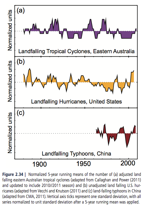
From AR5, wg I
Figure 3
Note that a more important metric than “how many?” is “how severe?” or a combination of both.
And for extra-tropical storms (i.e. outside the tropics), SREX p. 166:
In summary it is likely that there has been a poleward shift in the main Northern and Southern Hemisphere extratropical storm tracks during the last 50 years. There is medium confidence in an anthropogenic influence on this observed poleward shift. It has not formally been attributed.
There is low confidence in past changes in regional intensity.
And AR5, chapter 2, p. 217 & 220:
Some studies show an increase in intensity and number of extreme Atlantic cyclones (Paciorek et al., 2002; Lehmann et al., 2011) while others show opposite trends in eastern Pacific and North America (Gulev et al., 2001). Comparisons between studies are hampered because of the sensitivities in identification schemes and/ or different definitions for extreme cyclones (Ulbrich et al., 2009; Neu et al., 2012). The fidelity of research findings also rests largely with the underlying reanalyses products that are used..
..In summary, confidence in large scale changes in the intensity of extreme extratropical cyclones since 1900 is low. There is also low confidence for a clear trend in storminess proxies over the last century due to inconsistencies between studies or lack of long-term data in some parts of the world (particularly in the SH). Likewise, confidence in trends in extreme winds is low, owing to quality and consistency issues with analysed data.
Discussion
The IPCC SREX and AR5 reports were published in 2012 and 2013 respectively. There will be new research published since these reports analyzing the same data and possibly reaching different conclusions. When you have large decadal variability in poorly observed data with a small or non-existent trend then inevitably different groups will be able to reach different conclusions on these trends. And if you focus on specific regions you can demonstrate a clear and unmistakeable trend.
If you are looking for a soundbite just pick the right region.
The last 100 years have seen global warming. As this blog has made clear from the physics, more GHGs (all other things remaining equal) result in more warming. What proportion of the last 100 years is intrinsic climate variability vs the anthropogenic GHG proportion I have no idea.
The last century has seen no clear globally averaged change in floods, droughts or storms – as best as we can tell with very incomplete observing systems. Of course, some regions have definitely seen more, and some regions have definitely seen less. Whether this is different from the period from 1800-1900 or from 1700-1800 no one knows. Perhaps floods, droughts and tropical storms increased globally from 1700-1900. Perhaps they decreased. Perhaps the last 100 years have seen more variability. Perhaps not. (And in recognition of Poe’s law, I note that a few statements within the article presenting graphs did say the opposite of the graphs presented).
Articles in this Series
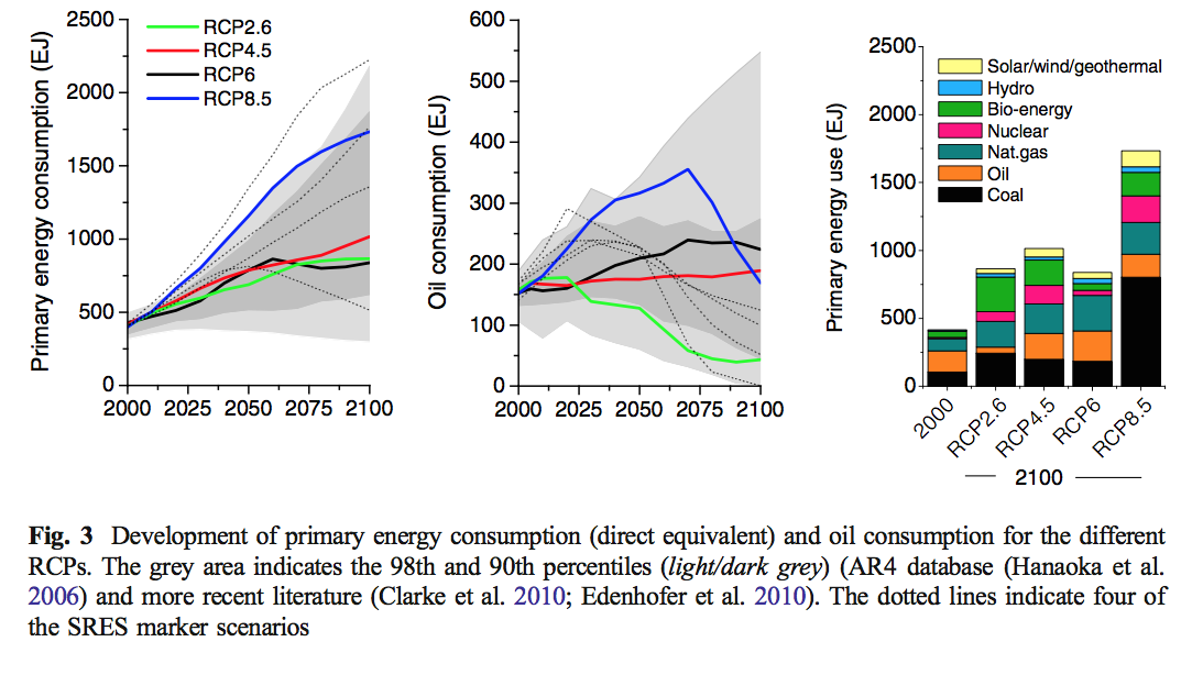
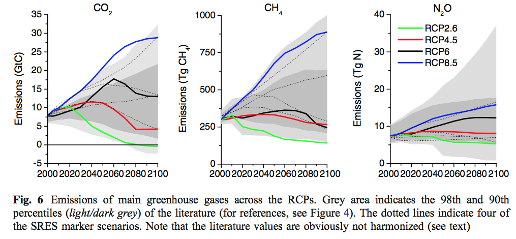
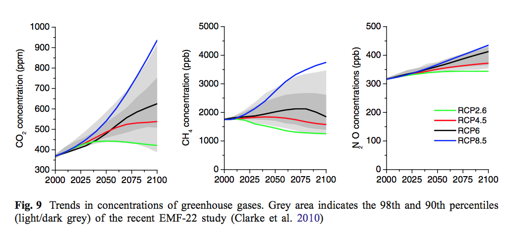
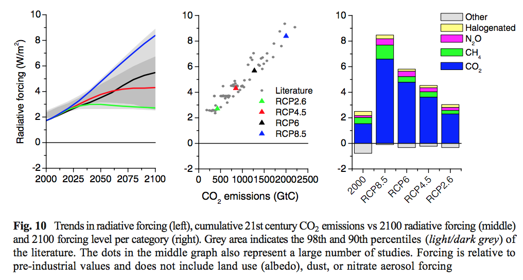
Impacts – II – GHG Emissions Projections: SRES and RCP
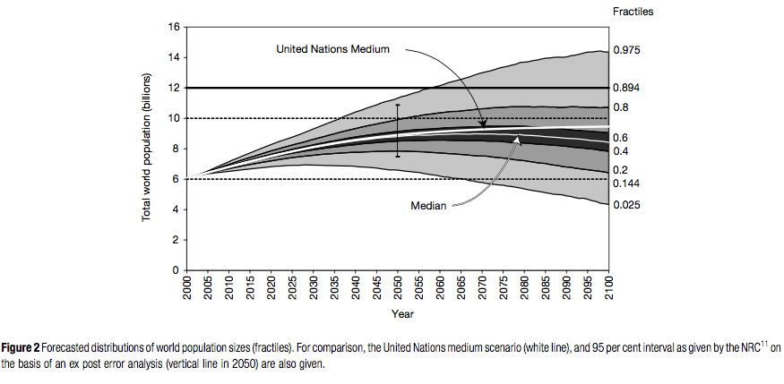
Impacts – III – Population in 2100
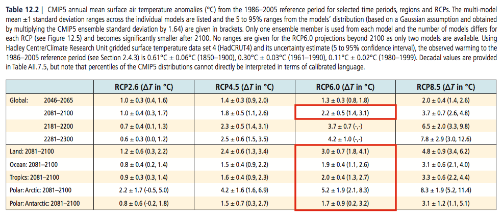
Impacts – IV – Temperature Projections and Probabilities
References
SREX = Managing the Risks of Extreme Events and Disasters to Advance Climate Change Adaptation Special Report, IPCC (2012)
Observations: Atmosphere and Surface. Chapter 2 of Working Group I to AR5, DL Hartmann et al (2013)
Global Trends and Variability in Soil Moisture and Drought Characteristics, 1950–2000, from Observation-Driven Simulations of the Terrestrial Hydrologic Cycle, Justin Sheffield & Eric Wood, Journal of Climate (2008) – free paper
Global warming and changes in drought, Kevin E Trenberth et al, Nature (2013) – free paper
Elusive drought: uncertainty in observed trends and short- and long-term CMIP5 projections, B Orlowsky & SI Seneviratne, Hydrology and Earth System Sciences (2013) – free paper


Impacts – I – Introduction
Posted in Commentary, Impacts on February 2, 2017| 18 Comments »
A long time ago, in About this Blog I wrote:
Now I would like to look at impacts of climate change. And so opinions and value judgements are inevitable.
In physics we can say something like “95% of radiation at 667 cm-1 is absorbed within 1m at the surface because of the absorption properties of CO2″ and be judged true or false. It’s a number. It’s an equation. And therefore the result is falsifiable – the essence of science. Perhaps in some cases all the data is not in, or the formula is not yet clear, but this can be noted and accepted. There is evidence in favor or against, or a mix of evidence.
As we build equations into complex climate models, judgements become unavoidable. For example, “convection is modeled as a sub-grid parameterization therefore..”. Where the conclusion following “therefore” is the judgement. We could call it an opinion. We could call it an expert opinion. We could call it science if the result is falsifiable. But it starts to get a bit more “blurry” – at some point we move from a region of settled science to a region of less-settled science.
And once we consider the impacts in 2100 it seems that certainty and falsifiability must be abandoned. “Blurry” is the best case.
Less than a year ago listening to America and the New Global Economy by Timothy Taylor (via audible.com) I remember he said something like “the economic cost of climate change was all lumped into a fat tail – if the temperature change was on the higher side”. Sorry for my inaccurate memory (and the downside of audible.com vs a real book). Well it sparked my interest in another part of the climate journey.
I’ve been reading IPCC Working Group II (wgII) – some of the “TAR” (= third assessment report) from 2001 for background and AR5, the latest IPCC report from 2014. Some of the impacts also show up in Working Group I which is about the physical climate science, and the IPCC Special Report on Managing the Risks of Extreme Events and Disasters to Advance Climate Change Adaptation from 2012, known as SREX (Special Report on Extremes). These are all available at the IPCC website.
The first chapter of the TAR, Working Group II says:
A couple of common complaints in the blogosphere that I’ve noticed are:
Within the field of papers and IPCC reports it’s clear that CO2 increasing plant growth is not ignored. Likewise, there are expected to be winners and losers (often, but definitely not exclusively, geographically distributed), even though the IPCC summarizes the expected overall effect as negative.
Of course, there is a highly entertaining field of “recycled press releases about the imminent catastrophe of climate change” which I’m sure ignores any positives or tradeoffs. Even in what could charitably be called “respected media outlets” there seem to be few correspondents with basic scientific literacy. Not even the ability to add up the numbers on an electricity bill or distinguish between the press release of a company planning to get wonderful results in 2025 vs today’s reality.
Anyway, entertaining as it is to shoot fish in a barrel, we will try to stay away from discussing newsotainment and stay with the scientific literature and IPCC assessments. Inevitably, we’ll stray a little.
I haven’t tried to do a comprehensive summary of the issues believed to impact humanity, but here are some:
Possibly I’ve missed some.
Covering the subject is not easy but it’s an interesting field.
Read Full Post »