Commentary | The Science of Doom

Archive for the ‘Commentary’ Category

The Debate is Over – 99% of Scientists believe Gravity and the Heliocentric Solar System so therefore..

Posted in Commentary on August 1, 2017| 171 Comments »

At least 99.9% of physicists believe the theory of gravity, and the heliocentric model of the solar system. The debate is over. There is no doubt that we can send a manned (and woman-ed) mission to Mars.

Some “skeptics” say it can’t be done. They are denying basic science! Gravity is plainly true. So is the heliocentric model. Everyone agrees. There is an overwhelming consensus. So the time for discussion is over. There is no doubt about the Mars mission.

I create this analogy (note 1) for people who don’t understand the relationship between five completely different ideas:

the “greenhouse” effect
burning fossil fuels adds CO2 to the atmosphere, increasing the “greehouse” effect
climate models
crop models
economic models

The first two items on the list are fundamental physics and chemistry, and while advanced to prove (see The “Greenhouse” Effect Explained in Simple Terms for the first one) to people who want to work through a proof, they are indisputable. Together they create the theory of AGW (anthropogenic global warming). This says that humans are contributing to global warming by burning fossil fuels.

99.9% of people who understand atmospheric physics believe this unassailable idea (note 2).

This means that if we continue with “business as usual” (note 3) and keep using fossil fuels to generate energy, then by 2100 the world will be warmer than today.

How much warmer?

For that we need climate models.

Climate Models

These are models which break the earth’s surface, ocean and atmosphere into a big grid so that we can use physics equations (momentum, heat transfer and others) to calculate future climate (this class of model is called finite element analysis). These models include giant fudge-factors that can’t be validated (by giant fudge factors I mean “sub-grid parameterizations” and unknown parameters, but I’m writing this article for a non-technical audience).

One way to validate models is to model the temperature over the last 100 years. Another way is to produce a current climatology that matches observations. Generally temperature is the parameter with most attention (note 4).

Some climate models predict that if we double CO2 in the atmosphere (from pre-industrial periods) then surface temperature will be around 4.5ºC warmer. Others that the temperature will be 1.5ºC warmer. And everything in between.

Surely we can just look at which models reproduced the last 100 years temperature anomaly the best and work with those?

From Mauritsen et al 2012

If the model that predicts 1.5ºC in 2100 is close to the past, while the one that predicts 4.5ºC has a big overshoot, we will know that 1.5ºC is a more likely future. Conversely, if the model that predicts 4.5ºC in 2100 is close to the past but the 1.5ºC model woefully under-predicts the last 100 years of warming then we can expect more like 4.5ºC in 2100.

You would think so, but you would be wrong.

All the models get the last 100 years of temperature changes approximately correct. Jeffrey Kiehl produced a paper 10 years ago which analyzed the then current class of models and gently pointed out the reason. Models with large future warming included a high negative effect from aerosols over the last 100 years. Models with small future warming included a small negative effect from aerosols over the last 100 years. So both reproduced the past but with a completely different value of aerosol cooling. You might think we can just find out the actual cooling effect of aerosols around 1950 and then we will know which climate model to believe – but we can’t. We didn’t have satellites to measure the cooling effect of aerosols back then.

This is the challenge of models with many parameters that we don’t know. When a modeler is trying to reproduce the past, or the present, they pick the values of parameters which make the model match reality as best as they can. This is a necessary first step (note 5).

So how warm will it be in 2100 if we double CO2 in the atmosphere?

Somewhat warmer

Models also predict rainfall, drought and storms. But they aren’t as good as they are at temperature. Bray and von Storch survey climate scientists periodically on a number of topics. Here is their response to:

How would you rate the ability of regional climate models to make 50 year projections of convective rain storms/thunder storms? (1 = very poor to 7 = very good)

Similar ratings are obtained for rainfall predictions. The last 50 years has seen no apparent global worsening of storms, droughts and floods, at least according to the IPCC consensus (see Impacts – V – Climate change is already causing worsening storms, floods and droughts).

Sea level is expected to rise between around 0.3m to 0.6m (see Impacts – VI – Sea Level Rise 1 and IX – Sea Level 4 – Sinking Megacities) – this is from AR5 of the IPCC (under scenario RCP6). I mention this because the few people I’ve polled thought that sea level was expected to be 5-10m higher in 2100.

Actual reports with uneventful projections don’t generate headlines.

Crop Models

Crop models build on climate models. Once we know rainfall, drought and temperature we can work out how this impacts crops.

Will we starve to death? Or will there be plentiful food?

Past predictions of disaster haven’t been very accurate, although they are wildly popular with generating media headlines and book sales, as Paul Ehrlich found to his benefit. But that doesn’t mean future predictions of disaster are necessarily wrong.

There are a number of problems with trying to answer the question.

Even if climate models could predict the global temperature, when it comes to a region the size of, say, northern California their accuracy is much lower. Likewise for rainfall. Models which produce similar global temperature changes often have completely different regional precipitation changes. For example, from the IPCC Special Report on Extremes (SREX), p. 154:

At regional scales, there is little consensus in GCM projections regarding the sign of future change in monsoon characteristics, such as circulation and rainfall. For instance, while some models project an intense drying of the Sahel under a global warming scenario, others project an intensification of the rains, and some project more frequent extreme events..

In a warmer world with more CO2 (helps some plants) and maybe more rainfall, or maybe less what can we expect out of crop yields? It’s not clear. The IPCC AR5 wg II, ch 7, p 496:

For example, interactions among CO2 fertilization, temperature, soil nutrients, O3, pests, and weeds are not well understood (Soussana et al., 2010) and therefore most crop models do not include all of these effects.

Of course, as climate changes over the next 80 years agricultural scientists will grow different crops, and develop new ones. In 1900, almost half the US population worked in farming. Today the figure is 2-3%. Agriculture has changed unimaginably.

In the left half of this graph we can see global crop yield improvements over 50 years (the right side is projections to 2050):

From Ray et al 2013

Economic Models

What will the oil price be in 2020? Economic models give you the answer. Well, they give you an answer. And if you consult lots of models they give you lots of different answers. When the oil price changes a lot, which it does from time to time, all of the models turn out to be wrong. Predicting future prices of commodities is very hard, even when it is of paramount concern for major economies, and even when a company could make vast profits from accurate prediction.

AR5 of the IPCC report, wg 2, ch 7, p.512, had this to say about crop prices in 2050:

Changes in temperature and precipitation, without considering effects of CO2, will contribute to increased global food prices by 2050, with estimated increases ranging from 3 to 84% (medium confidence). Projections that include the effects of CO2 changes, but ignore O3 and pest and disease impacts, indicate that global price increases are about as likely as not, with a range of projected impacts from –30% to +45% by 2050..

..One lesson from recent model intercomparison experiments (Nelson et al., 2014) is that the choice of economic model matters at least as much as the climate or crop model for determining price response to climate change, indicating the critical role of economic uncertainties for projecting the magnitude of price impacts.

In 2001, the 3rd report (often called TAR) said, ch 5, p.238, perhaps a little more clearly:

..it should be noted however that hunger estimates are based on the assumptions that food prices will rise with climate change, which is highly uncertain

Economic models are not very good at predicting anything. As Herbert Stein said, summarizing a lifetime in economics:

Economists do not know very much
Other people, including the politicians who make economic policy, know even less about economics than economists do

Conclusion

Recently a group, Cook et al 2013, reviewed over 10,000 abstracts of climate papers and concluded that 97% believed in the proposition of AGW – the proposition that humans are contributing to global warming by burning fossil fuels. I’m sure if the question were posed the right way directly to thousands of climate scientists, the number would be over 99%.

It’s not in dispute.

AGW is a necessary theory for Catastrophic Anthropogenic Global Warming (CAGW). But not sufficient by itself.

Likewise we know for sure that gravity is real and the planets orbit the sun. But it doesn’t follow that we can get humans safely to Mars and back. Maybe we can. Understanding gravity and the heliocentric theory is a necessary condition for the mission, but a lot more needs to be demonstrated.

The uncertainties in CAGW are huge.

Economic models that have no predictive skill are built on limited crop models which are built on climate models which have a wide range of possible global temperatures and no consensus on regional rainfall.

Human ingenuity somehow solved the problem of going from 2.5bn people in the middle of the 20th century to more than 7bn people today, and yet the proportion of the global population in abject poverty (note 6) has dropped from over 40% to maybe 15%. This was probably unimaginable 70 years ago.

Perhaps reasonable people can question if climate change is definitely the greatest threat facing humanity?

Perhaps questioning the predictive power of economic models is not denying science?

Perhaps it is ok to be unsure about the predictive power of climate models that contain sub-grid parameterizations (giant fudge factors) and that collectively provide a wide range of forecasts?

Perhaps people who question the predictions aren’t denying basic (or advanced) science, and haven’t lost their reason or their moral compass?

—-

[Note to commenters, added minutes after this post was written – this article is not intended to restart debate over the “greenhouse” effect, please post your comments in one of the 10s (100s?) of articles that have covered that subject, for example – The “Greenhouse” Effect Explained in Simple Terms – Comments on the reality of the “greenhouse” effect posted here will be deleted. Thanks for understanding.]

References

Twentieth century climate model response and climate sensitivity, Jeffrey Kiehl (2007)

Tuning the climate of a global model, Mauritsen et al (2012)

Yield Trends Are Insufficient to Double Global Crop Production by 2050, Deepak K. Ray et al (2013)

Quantifying the consensus on anthropogenic global warming in the scientific literature, Cook et al, Environmental Research Letters (2013)

The Great Escape, Angus Deaton, Princeton University Press (2013)

The various IPCC reports cited are all available at their website

Notes

1. An analogy doesn’t prove anything. It is for illumination.

2. How much we have contributed to the last century’s warming is not clear. The 5th IPCC report (AR5) said it was 95% certain that more than 50% of recent warming was caused by human activity. Well, another chapter in the same report suggested that this was a bogus statistic and I agree, but that doesn’t mean I think that the percentage of warming caused by human activity is lower than 50%. I have no idea. It is difficult to assess, likely impossible. See Natural Variability and Chaos – Three – Attribution & Fingerprints for more.

3. Reports on future climate often come with the statement “under a conservative business as usual scenario” but refer to a speculative and hard to believe scenario called RCP8.5 – see Impacts – II – GHG Emissions Projections: SRES and RCP. I think RCP 6 is much closer to the world of 2100 if we do little about carbon emissions and the world continues on the kind of development pathways that we have seen over the last 60 years. RCP8.5 was a scenario created to match a possible amount of CO2 in the atmosphere and how we might get there. Calling it “a conservative business as usual case” is a value-judgement with no evidence.

4. More specifically the change in temperature gets the most attention. This is called the “temperature anomaly”. Many models that do “well” on temperature anomaly actually do quite badly on the actual surface temperature. See Models, On – and Off – the Catwalk – Part Four – Tuning & the Magic Behind the Scenes – you can see that many “fit for purpose” models have current climate halfway to the last ice age even though they reproduce the last 100 years of temperature changes pretty well. That is, they model temperature changes quite well, but not temperature itself.

5. This is a reasonable approach used in modeling (not just climate modeling) – the necessary next step is to try to constrain the unknown parameters and giant fudge factors (sub-grid parameterizations). Climate scientists work very hard on this problem. Many confused people writing blogs think that climate modelers just pick the values they like, produce the model results and go have coffee. This is not the case, and can easily be seen by just reviewing lots of papers. The problem is well-understood among climate modelers. But the world is a massive place, detailed past measurements with sufficient accuracy are mostly lacking, and sub-grid parameterizations of non-linear processes are a very difficult challenge (this is one of the reasons why turbulent flow is a mostly unsolved problem).

6. This is a very imprecise term. I refer readers to the 2015 Nobel Prize winner Angus Deaton and his excellent book, The Great Escape (2013) for more.

Read Full Post »

The Confirmation Bias – a Feature not a Bug

Posted in Commentary on June 25, 2017| 51 Comments »

A long time ago I wrote The Confirmation Bias – Or Why None of Us are Really Skeptics, with a small insight from Nassim Taleb. Right now I’m rereading The Righteous Mind: Why Good People are Divided by Politics and Religion by Jonathan Haidt.

This is truly a great book if you want to understand more about how we think and how we delude ourselves. Through experiments cognitive psychologists demonstrate that once our “moral machinery” has clicked in, which happens very easily, our reasoning is just an after-the-fact rationalization of what we already believe.

Haidt gives the analogy of a rider on an elephant. The elephant starts going one way rather than another, and the rider, unaware of why, starts coming up with invented reasons for the new direction. It’s like the rider is the PR guy for the elephant. In Haidt’s analogy, the rider is our reasoning, and the elephant is our moral machinery. The elephant is in charge. The rider thinks he is.

An an intuitionist, I’d say that the worship of reason is itself an illustration of one of the most long-lived delusions in Western history: the rationalist delusion..

..The French cognitive scientists Hugo Mercier and Dan Sperber recently reviewed the vast research literature on motivated reasoning (in social psychology) and on the biases and errors of reasoning (in cognitive psychology). They concluded that most of the bizarre and depressing research findings make perfect sense once you see reasoning as having evolved not to help us find truth but to help us engage in arguments, persuasion and manipulation in the context of discussions with other people.

As they put it, “skilled arguers ..are not after the truth but after arguments supporting their views.” This explains why the confirmation bias is so powerful and so ineradicable. How hard could it be to teach students to look on the other side, to look for evidence against their favored view? Yet it’s very hard, and nobody has yet found a way to do it. It’s hard because the confirmation bias is a built-in feature (of an argumentative mind), not a bug that can be removed (from a platonic mind)..

..In the same way, each individual reasoner is really good at one thing: finding evidence to support the position he or she already holds, usually for intuitive reasons..

..I have tried to make a reasoned case that our moral capacities are best described from an intuitionist perspective. I do not claim to have examined the question from all sides, nor to have offered irrefutable proof.

Because of the insurmountable power of the confirmation bias, counterarguments will have to be produced by those who disagree with me.

Haidt also highlights some research showing that more intelligence and education makes you better at generating more arguments for your side of the argument, but not for finding reasons on the other side. “Smart people make really good lawyers and press secretaries.. people invest their IQ in buttressing their own case rather than in exploring the entire issue more fully and evenhandedly.”

The whole book is very readable and full of studies and explanations.

If you fancy a bucket of ice cold water thrown over the rationalist delusion then this is a good way to get it.

Read Full Post »

Impacts – VIII – Sea level 3 – USA

Posted in Commentary, Impacts on February 19, 2017| 101 Comments »

In Parts VI and VII we looked at past and projected sea level rise. It is clear that the sea level has risen over the last hundred years, and it’s clear that with more warming sea level will rise some more. The uncertainties (given a specific global temperature increase) are more around how much more ice will melt than how much the ocean will expand (warmer water expands). Future sea level rise will clearly affect some people in the future, but very differently in different countries and regions. This article considers the US.

A month or two ago, via a link from a blog, I found a paper which revised upwards a current calculation (or average of such calculations) of damage due to sea level rise in 2100 in the US. Unfortunately I can’t find the paper, but essentially the idea was people would continue moving to the ocean in ever increasing numbers, and combined with possible 1m+ sea level rise (see Part VI & VII) the cost in the US would be around $1TR (I can’t remember the details but my memory tells me this paper concluded costs were 3x previous calculations due to this ever increasing population move to coastal areas – in any case, the exact numbers aren’t important).

Two examples that I could find (on global movement of people rather than just in the US), Nicholls 2011:

..This threatened population is growing significantly (McGranahan et al., 2007), and it will almost certainly increase in the coming decades, especially if the strong tendency for coastward migration continues..

And Anthoff et al 2010

Fifthly, building on the fourth point, FUND assumes that the pattern of coastal development persists and attracts future development. However, major disasters such as the landfall of hurricanes could trigger coastal abandonment, and hence have a profound influence on society’s future choices concerning coastal protection as the pattern of coastal occupancy might change radically.

A cycle of decline in some coastal areas is not inconceivable, especially in future worlds where capital is highly mobile and collective action is weaker. As the issue of sea-level rise is so widely known, disinvestment from coastal areas may even be triggered without disasters..

I was struck by the “trillion dollar problem” paper and the general issues highlighted in other papers. The future cost of sea level rise in the US is not just bad, it’s extremely expensive because people will keep moving to the ocean.

Why are people moving to the coast?

So here is an obvious take on the subject that doesn’t need an IAM (integrated assessment model).. Perhaps lots of people missed the IPCC TAR (third assessment report) in 2001. Perhaps anthropogenic global warming fears had not reached a lot of the population. Maybe it didn’t get a lot of media coverage. But surely no could have missed Al Gore’s movie. I mean, I missed it from choice, but how could anyone in rich countries not know about the discussion?

So anyone since 2006 (arbitrary line in the sand) who bought a house that is susceptible to sea level rise is responsible for their own loss that they incur around 2100. That is, if the worst fears about sea level rise play out, combined with more extreme storms (subject of a future article) which create larger ocean storm surges, their house won’t be worth much in 2100.

Now, barring large increases in life expectancy, anyone who bought a house in 2005 will almost certainly be dead in 2100. There will be a few unlucky centenarians.

Think of it as an estate tax. People who have expensive ocean-front houses will pass on their now worthless house to their children or grandchildren. Some people love the idea of estate taxes – in that case you have a positive. Some people hate the idea of estate taxes – in that case strike it up as a negative. And, drawing a long bow here, I suspect a positive correlation between concern about climate change and belief in the positive nature of estate taxes, so possibly it’s a win-win for many people.

Now onto infrastructure.

From time to time I’ve had to look at depreciation and official asset life for different kinds of infrastructure and I can’t remember seeing one for 100 years. 50 years maybe for civil structures. I’m definitely not an expert. That said, even if the “official depreciation” gives something a life of 50 years, much is still being used 150 years later – buildings, railways, and so on.

So some infrastructure very close to the ocean might have to be abandoned. But it will have had 100 years of useful life and that is pretty good in public accounting terms.

Why is anyone building housing, roads, power stations, public buildings, railways and airports in the US in locations that will possibly be affected by sea level rise in 2100? Maybe no one is.

So the cost of sea level rise for 2100 in the US seems to be a close to zero cost problem.

These days, if a particular area is recognized as a flood plain people are discouraged from building on it and no public infrastructure gets built there. It’s just common sense.

Some parts of New Orleans were already below sea level when Hurricane Katrina hit. Following that disaster, lots of people moved out of New Orleans to a safer suburb. Lots of people stayed. Their problems will surely get worse with a warmer climate and a higher sea level (and also if storms gets stronger – subject of a future article). But they already had a problem. Infrastructure was at or below sea level and sufficient care was not taken of their coastal defences.

A major problem that happens overnight, or over a year, is difficult to deal with. A problem 100 years from now that affects a tiny percentage of the land area of a country, even with a large percentage (relatively speaking) of population living there today, is a minor problem.

Perhaps the costs of recreating current threatened infrastructure a small distance inland are very high, and the existing infrastructure would in fact have lasted more than 100 years. In that case, people who believe Keynesian economics might find the economic stimulus to be a positive. People who don’t think Keynesian economics does anything (no multiplier effect) except increase taxes, or divert productive resources into less productive resources will find it be a negative. Once again, drawing a long bow, I see a correlation between people more concerned about climate change also being more likely to find Keynesian economics a positive. Perhaps again, there is a win-win.

In summary, given the huge length of time to prepare for it, US sea level rise seems like a minor planning inconvenience combined with an estate tax.

Articles in this Series

Impacts – I – Introduction

Impacts – II – GHG Emissions Projections: SRES and RCP

Impacts – III – Population in 2100

Impacts – IV – Temperature Projections and Probabilities

Impacts – V – Climate change is already causing worsening storms, floods and droughts

Impacts – VI – Sea Level Rise 1

Impacts – VII – Sea Level 2 – Uncertainty

References

Planning for the impacts of sea level rise, RJ Nicholls, Oceanography (2011)

The economic impact of substantial sea-level rise, David Anthoff et al, Mitig Adapt Strateg Glob Change (2010)

Read Full Post »

Impacts – I – Introduction

Posted in Commentary, Impacts on February 2, 2017| 18 Comments »

A long time ago, in About this Blog I wrote:

Opinions
Opinions are often interesting and sometimes entertaining. But what do we learn from opinions? It’s more useful to understand the science behind the subject. What is this particular theory built on? How long has the theory been “established”? What lines of evidence support this theory? What evidence would falsify this theory? What do opposing theories say?

Now I would like to look at impacts of climate change. And so opinions and value judgements are inevitable.

In physics we can say something like “95% of radiation at 667 cm^-1 is absorbed within 1m at the surface because of the absorption properties of CO2″ and be judged true or false. It’s a number. It’s an equation. And therefore the result is falsifiable – the essence of science. Perhaps in some cases all the data is not in, or the formula is not yet clear, but this can be noted and accepted. There is evidence in favor or against, or a mix of evidence.

As we build equations into complex climate models, judgements become unavoidable. For example, “convection is modeled as a sub-grid parameterization therefore..”. Where the conclusion following “therefore” is the judgement. We could call it an opinion. We could call it an expert opinion. We could call it science if the result is falsifiable. But it starts to get a bit more “blurry” – at some point we move from a region of settled science to a region of less-settled science.

And once we consider the impacts in 2100 it seems that certainty and falsifiability must be abandoned. “Blurry” is the best case.

Less than a year ago listening to America and the New Global Economy by Timothy Taylor (via audible.com) I remember he said something like “the economic cost of climate change was all lumped into a fat tail – if the temperature change was on the higher side”. Sorry for my inaccurate memory (and the downside of audible.com vs a real book). Well it sparked my interest in another part of the climate journey.

I’ve been reading IPCC Working Group II (wgII) – some of the “TAR” (= third assessment report) from 2001 for background and AR5, the latest IPCC report from 2014. Some of the impacts also show up in Working Group I which is about the physical climate science, and the IPCC Special Report on Managing the Risks of Extreme Events and Disasters to Advance Climate Change Adaptation from 2012, known as SREX (Special Report on Extremes). These are all available at the IPCC website.

The first chapter of the TAR, Working Group II says:

The world community faces many risks from climate change. Clearly it is important to understand the nature of those risks, where natural and human systems are likely to be most vulnerable, and what may be achieved by adaptive responses. To understand better the potential impacts and associated dangers of global climate change, Working Group II of the Intergovernmental Panel on Climate Change (IPCC) offers this Third Assessment Report (TAR) on the state of knowledge concerning the sensitivity, adaptability, and vulnerability of physical, ecological, and social systems to climate change.

A couple of common complaints in the blogosphere that I’ve noticed are:

“all the impacts are supposed to be negative but there are a lot of positives from warming”
“CO2 will increase plant growth so we’ll be better off”

Within the field of papers and IPCC reports it’s clear that CO2 increasing plant growth is not ignored. Likewise, there are expected to be winners and losers (often, but definitely not exclusively, geographically distributed), even though the IPCC summarizes the expected overall effect as negative.

Of course, there is a highly entertaining field of “recycled press releases about the imminent catastrophe of climate change” which I’m sure ignores any positives or tradeoffs. Even in what could charitably be called “respected media outlets” there seem to be few correspondents with basic scientific literacy. Not even the ability to add up the numbers on an electricity bill or distinguish between the press release of a company planning to get wonderful results in 2025 vs today’s reality.

Anyway, entertaining as it is to shoot fish in a barrel, we will try to stay away from discussing newsotainment and stay with the scientific literature and IPCC assessments. Inevitably, we’ll stray a little.

I haven’t tried to do a comprehensive summary of the issues believed to impact humanity, but here are some:

sea level rise
heatwaves
droughts
floods
more powerful cyclones and storms
food production
ocean acidification
extinction of animal and plant species
more pests (added, thanks Tom, corrected thanks DeWitt)
disease (added, thanks Tom)

Possibly I’ve missed some.

Covering the subject is not easy but it’s an interesting field.

Read Full Post »

Renewable Energy I

Posted in Commentary, Renewables on July 30, 2015| 122 Comments »

This blog is about climate science.

I wanted to take a look at Renewable Energy because it’s interesting and related to climate science in an obvious way. Information from media sources confirms my belief that 99% of what is produced by the media is rehashed press releases from various organizations with very little fact checking. (Just a note for citizens alarmed by this statement – they are still the “go to source” for the weather, footage of disasters and partly-made-up stories about celebrities).

Regular readers of this blog know that the articles and discussion so far have only been about the science – what can be proven, what evidence exists, and so on. Questions about motives, about “things people might have done”, and so on, are not of interest in the climate discussion (not for this blog). There are much better blogs for that – with much larger readerships.

Here’s an extract from About this Blog:

Opinions
Opinions are often interesting and sometimes entertaining. But what do we learn from opinions? It’s more useful to understand the science behind the subject. What is this particular theory built on? How long has the theory been “established”? What lines of evidence support this theory? What evidence would falsify this theory? What do opposing theories say?
Anything else?
This blog will try and stay away from guessing motives and insulting people because of how they vote or their religious beliefs. However, this doesn’t mean we won’t use satire now and again as it can make the day more interesting.

The same principles will apply for this discussion about renewables. Our focus will be on technical and commercial aspects of renewable energy, with a focus on evidence rather than figuring it out from “motive attribution”. And wishful thinking – wonderful though it is for reducing personal stress – will be challenged.

As always, the moderator reserves the right to remove comments that don’t meet these painful requirements.

Here’s a claim about renewables from a recent media article:

By Bloomberg New Energy Finance’s most recent calculations a new wind farm in Australia would cost $74 a megawatt hour..

..”Wind is already the cheapest, and solar PV [photovoltaic panels] will be cheaper than gas in around two years, in 2017. We project that wind will continue to decline in cost, though at a more modest rate than solar. Solar will become the dominant source in the longer term.”

I couldn’t find any evidence in the article that verified the claim. Only that it came from Bloomberg New Energy Finance and was the opposite of a radio shock jock. Generally I favor my dogs’ opinions over opinionated media people (unless it is about the necessity of an infinite supply of Schmackos starting now, right now). But I have a skeptical mindset and not knowing the wonderful people at Bloomberg I have no idea whether their claim is rock-solid accurate data, or “wishful thinking to promote their products so they can make lots of money and retire early”.

Calculating the cost of anything like this is difficult. What is the basis of the cost calculation? I don’t know if the claim in BNEF’s calculation is “accurate” – but without context it is not such a useful number. The fact that BNEF might have some vested interest in a favorable comparison over coal and gas is just something I assume.

But, like with climate science, instead of discussing motives and political stances, we will just try and figure out how the numbers stack up. We won’t be pitting coal companies (=devils or angels depending on your political beliefs) against wind turbine producers (=devils or angels depending on your political beliefs) or against green activists (=devils or angels depending on your political beliefs).

Instead we will look for data – a crazy idea and I completely understand how very unpopular it is. Luckily, I’m sure I can help people struggling with the idea to find better websites on which to comment.

Calculating the Cost

I’ve read the details of a few business plans and I’m sure that most other business plans also have the same issue – change a few parameters (=”assumptions”, often “reasonable assumptions”) and the outlook goes from amazing riches to destitution and bankruptcy.

The cost per MWHr of wind energy will depend on a few factors:

cost of buying a wind turbine
land acquisition/land rental costs
installation cost
grid connection costs
the “backup requirement” aka “capacity credit”
cost of capital
lifetime of equipment
maintenance costs
% utilization (output energy / nameplate capacity)

And of course, in any discussion about “the future”, favorable assumptions can be made about “the next generation”. Is the calculation of $74/MWHr based on what was shipped 5 years ago and its actuals, or what is suggested for a turbine purchased next year?

If you want wind to look better than gas or coal – or the converse – there are enough variables to get the result you want. I’ll be amazed if you can’t change the relative costs by a factor of 5 by playing around with what appear to be reasonable assumptions.

Perhaps the data is easy to obtain. I’m sure many readers have some or all of this data to hand.

Moore’s Law and Other Industries

Most people are familiar with the now legendary statement from the 1960s about semiconductor performance doubling every 18 months. This revolution is amazing. But it’s unusual.

There are a lot of economies of scale from mass production in a factory. But mostly limiting cases are reached pretty quickly, after which cost reductions of a few percent a year are great results – rather than producing the same product for 1% of what it cost just 10 years before. Semiconductors are the exception.

When a product is made from steel alloys, carbon fiber composites or similar materials we can’t expect Moore’s law to kick in. On the other hand, products that rely on a combination of software, electronic components and “traditional materials” and have been produced on small scales up until now can expect major cost reductions from amortizing costs (software, custom chips, tooling, etc) and general economies of scale (purchasing power, standardizing processes, etc).

In some industries, rapid growth actually causes cost increases. If you want an experienced team to provide project management, installation and commissioning services you might find that the boom in renewables is driving those costs up, not down.

A friend of mine working for a natural gas producer in Queensland, Australia recounted the story of the cost of building a dam a few years ago. Long story short, the internal estimates ranged from $2M to $7M, but when the tenders came in from general contractors the prices were $10M to $25M. The reason was a combination of:

escalating contractor costs (due to the boom)
compliance with new government environmental regulations
compliance with the customer’s many policies / OH&S requirements
the contractual risk due to all of the above, along with the significant proliferation of contract terms (i.e., will we get sued, have we taken on liabilities we don’t understand, etc)

The point being that industry insiders – i.e., the customer – with a strong vested interest in understanding current costs was out by a factor of more than three in a traditional enterprise. This kind of inaccuracy is unusual but it can happen when the industry landscape is changing quickly.

Even if you have signed a fixed price contract with an EPC you can only be sure this is the minimum you will be paying.

The only point I’m making is that a lot of costs are unknown even by experienced people in the field. Companies like BNEF might make some assumptions but it’s a low stress exercise when someone else will be paying the actual bills.

Intermittency & Grid Operators

We will discuss this further in future articles. This is a key issue between renewables and fossil fuel / nuclear power stations. The traditional power stations can create energy when it is needed. Wind and solar – mainstays of the renewable revolution – create energy when the sun shines and the wind blows.

As a starting point for any discussion let’s assume that storing energy is massively uneconomic. While new developments might be available “around the corner”, storing energy is very expensive. The only real mechanism is pumped hydro schemes. Of course, we can discuss this.

Grid operators have a challenge – balance demand with supply (because storage capacity is virtually zero). Demand is variable and although there is some predictability, there are unexpected changes even in the short term.

The demand curve depends on the country. For example, the UK has peak demand in the winter evenings. Wealthy hotter countries have peak demand in the summer in the middle of the day (air-conditioning).

There are two important principles:

Grid operators already have to deal with intermittency because conventional power stations go off-line with planned outages and with unplanned, last minute, outages
Renewables have a “capacity credit” that is usually less than their expected output

The first is a simple one. An example is the Sizewell B nuclear power station in the UK supplying about 1GW [fixed] out of 80GW of total grid supply. From time to time it shuts down and the grid operator gets very little notice. So grid operators already have to deal with this. They use statistical calculations to ensure excess supply during normal operation, based on an acceptable “loss of load probability”. Total electricity demand is variable and supply is continually adjusted to match that demand. Of course, the scale of intermittency from large penetration of renewables may present challenges that are difficult to deal with by comparison with current intermittency.

The second is the difficult one. Here’s an example from a textbook by Godfrey, that’s actually a collection of articles on (mainly) UK renewables:

The essence of the calculation is a probabilistic one. At small penetration levels, the energy input from wind power displaces the need for energy generation from traditional sources. But as the percentage of wind power increases, the “potential down time” causes more problems – requiring more backup generation on standby. In the calculations above, wind going from 0.5 GW to 25 GW only saves 4 GW in conventional “capacity”. This is the meaning of capacity credit – adding 25 GW of wind power (under this simulation) provides a capacity credit of only 4 GW. So you can’t remove 25 GW of conventional from the grid, you can only remove 4 GW of conventional power.

Now the calculation of capacity credit depends on the specifics of the history of wind speeds in the region. Increasing the geographical spread of wind power generation produces better results, dependent on the lower correlation of wind speeds across larger regions. Different countries get different results.

So there’s an additional cost with wind power that someone has to pay for – which increases along with the penetration of wind power. In the immediate future this might not be a problem because perhaps the capacity already exists and is just being put on standby. However, at some stage these older plants will be at end of life and conventional plants will need to be built to provide backup.

Many calculations exist of the estimated $/MWh from providing such a backup. We will dig into those in future articles. My initial impression is that there are a lot of unknowns in the real cost of backup supply because for much potential backup supply the lifetime / maintenance impact of frequent start-stops is unclear. A lot of this is thermal shock issues – each thermal cycle costs $X.. (based on the design of the plant to handle so many thousand starts before a major overhaul is needed).

The Other Side of the Equation – Conventional Power

It will also be interesting to get some data around conventional power. Right now, the cost of displacing conventional power is new investment in renewables, but keeping conventional power is not free. Every existing station has a life and will one day need to be replaced (or demand will need to be reduced). It might be a deferred cost but it will still be a cost.

$ and GHG emissions

There is a cost to adding 1GW of wind power. There is a cost to adding 1GW of solar power. There is also a GHG cost – that is, building a solar panel or a wind turbine is not energy free and must be producing GHGs in the process. It would be interesting to get some data on this also.

Conclusion – Introduction

I wrote this article because finding real data is demanding and many websites focused on the topic are advocacy-based with minimal data. Their starting point is often the insane folly and/or mendacious intent of “the other side”. The approach we will take here is to gather and analyze data.. As if the future of the world was not at stake. As if it was not a headlong rush into lunacy to try and generate most energy from renewables.. As if it was not an unbelievable sin to continue to create electricity from fossil fuels..

This approach might allow us to form conclusions from the data rather than the reverse.

Let’s see how this approach goes.

I am hoping many current (and future) readers can contribute to the discussion – with data, uncertainties, clarifications.

I’m not expecting to be able to produce “a number” for windpower or solar power. I’m hopeful that with some research, analysis and critical questions we might be able to summarize some believable range of values for the different elements of building a renewable energy supply, and also quantify the uncertainties.

Most of what I will write in future articles I don’t yet know. Perhaps someone already has a website where this project is already complete and in my Part Two will just point readers there..

Articles in this Series

Renewable Energy I – Introduction

Renewables II – Solar and Free Lunches – Solar power

Renewables III – US Grid Operators’ Opinions – The grid operators’ concerns

Renewables IV – Wind, Forecast Horizon & Backups – Some more detail about wind power – what do we do when the wind goes on vacation

Renewables V – Grid Stability As Wind Power Penetration Increases

Renewables VI – Report says.. 100% Renewables by 2030 or 2050

Renewables VII – Feasibility and Reality – Geothermal example

Renewables VIII – Transmission Costs And Outsourcing Renewable Generation

Renewables IX – Onshore Wind Costs

Renewables X – Nationalism vs Inter-Nationalism

Renewables XI – Cost of Gas Plants vs Wind Farms

Renewables XII – Windpower as Baseload and SuperGrids

Renewables XIII – One of Wind’s Hidden Costs

Renewables XIV – Minimized Cost of 99.9% Renewable Study

Renewables XV – Offshore Wind Costs

Renewables XVI – JP Morgan advises

Renewables XVII – Demand Management 1

Renewables XVIII – Demand Management & Levelized Cost

Renewables XIX – Behind the Executive Summary and Reality vs Dreams

References

Renewable Electricity and the Grid : The Challenge of Variability, Godfrey Boyle, Earthscan (2007)

Read Full Post »

The Holocaust, Climate Science and Proof

Posted in Commentary on February 4, 2015| 558 Comments »

I’ve been a student of history for a long time and have read quite a bit about Nazi Germany and WWII. In fact right now, having found audible.com I’m listening to an audio book The Coming of the Third Reich, by Richard Evans, while I walk, drive and exercise.

It’s heartbreaking to read about the war and to read about the Holocaust. Words fail me to describe the awfulness of that regime and what they did.

But it’s pretty easy for someone who is curious about evidence, or who has had someone question whether or not the Holocaust actually took place, to find and understand the proof.

The photos. The bodies. The survivors’ accounts. The thousands of eyewitness accounts. The army reports. The stated aims of Hitler and many of the leading Nazis in their own words.

We can all understand how to weigh up witness accounts and photos. It’s intrinsic to our nature.

People who don’t believe the Nazis murdered millions of Jews are denying simple and overwhelming evidence.

Let’s compare that with the evidence behind the science of anthropogenic global warming (AGW) and the inevitability of a 2-6ºC rise in temperature if we continue to add CO2 and other GHGs to the atmosphere.

Step 1 – The ‘greenhouse’ effect

To accept AGW of course you need to accept the ‘greenhouse’ effect. It’s fundamental science and not in question but what if you don’t take my word for it? What if you want to check for yourself?

And by the way, the complexity of the subject for many people becomes clear even at this stage, with countless hordes not even clear that the ‘greenhouse’ effect is a just a building block for AGW. It is not itself AGW.

AGW relies on the ‘greenhouse’ effect but also on other considerations.

I wrote The “Greenhouse” Effect Explained in Simple Terms to make it simple, yet not too simple. But that article relies on (and references) many basics – radiation, absorption and emission of radiation through gases, heat transfer and convection. All of those are necessary to understand the greenhouse effect.

Many people have conceptual misunderstandings of “basic” physics. In reading comments on this blog and on other blogs I often see fundamental misunderstanding of how heat transfer works. No space here for that.

But the difficulty of communicating a physics idea is very real. Once someone has a conceptual block because they think some process works a subtly different way, the only way to resolve the question is with equations. It is further complicated because these misunderstandings are often unstated by the commenter – they don’t realize they see the world differently from physics basics.

So when we need to demonstrate that the greenhouse effect is real, and that it increases with more GHGs we need some equations. And by ‘increases’ I mean more GHGs mean a higher surface temperature, all other things being equal. (Which, of course, they never are).

The equations are crystal clear and no one over the age of 10 could possibly be confused. I show the equations for radiative transfer (and their derivation) in Understanding Atmospheric Radiation and the “Greenhouse” Effect – Part Six – The Equations:

I_λ(0) = I_λ(τ_m)e^-τ_m + ∫ B_λ(T)e^-τ dτ [16]

The terms are explained in that article. In brief, the equation shows how the intensity of radiation at the top of the atmosphere at one wavelength is affected by the number of absorbing molecules in the atmosphere. And, obviously, you have to integrate it over all wavelengths. Why do I even bring that up, it’s so simple?

Voila.

And equally obviously, anyone questioning the validity of the equation, or the results from the equation, is doing so from evil motives.

I do need to add that we have to prescribe the temperature profile in the atmosphere (and the GHG concentration) to be able to solve this equation. The temperature profile is known as the lapse rate – temperature reduces as you go up in altitude. In the tropical regions where convection is stronger we can come up with a decent equation for the lapse rate.

All you have to know is the first law of thermodynamics, the ideal gas law and the equation for the change in pressure vs height due to the mass of the atmosphere. Everyone can do this in their heads of course. But here it is:

So with these two elementary principles we can prove that more GHGs means a higher surface temperature before any feedbacks. That’s the ‘greenhouse’ effect.

Step 2 – AGW = ‘Greenhouse effect’ plus feedbacks

This is so simple. Feedbacks are things like – a hotter world probably has more water vapor in the atmosphere, and water vapor is the most important GHG, so this amplifies the ‘greenhouse’ effect of increasing CO2. Calculating the changes is only a little more difficult than the super simple equations I showed earlier.

You just need a GCM – a climate model run on a supercomputer. That’s all.

There are many misconceptions about climate models but only people who are determined to believe a lie can possibly believe them.

As an example, many people think that the amplifying effect, or positive feedback, of water vapor is programmed into the GCMs. All they have to do is have a quick read through the 200-page technical summary of a model like say CAM (community atmosphere model).

Here is an extract from Description of the NCAR Community Atmosphere Model (CAM 3.0), W.D. Collins (2004):

As soon as anyone reads this – and if they can’t be bothered to find the reference via Google Scholar and read it, well, what can you say about such people – as soon as they read it, of course, it’s crystal clear that positive feedback isn’t “programmed in” to climate models.

So GCMs all come to the conclusion that more GHGs results in a hotter world (2-6ºC). They solve basic physics equations in a “grid” fashion, stepping forward in time, and so the result is clear and indisputable.

Step 3 – Attribution Studies

I recently spent some time reading AR4 and AR5 (the IPCC reports) on Attribution (Natural Variability and Chaos – Seven – Attribution & Fingerprints Or Shadows? and Natural Variability and Chaos – Three – Attribution & Fingerprints).

This is the work of attributing the last century’s rise in temperature to the increases in anthropogenic GHGs. I followed the trail of papers back and found one of the source papers by Hasselmann from 1993. In it we can clearly see the basis for attribution studies:

Now it’s very difficult to believe that anyone questioning attribution studies isn’t of evil intent. After all, there is the basic principle in black and white. Who could be confused?

As a side note, to excuse my own irredeemable article on the topic, the actual basis of attribution isn’t just in these equations, it is also in the assumption that climate models accurately calculate the statistics of natural variability. The IPCC chapter on attribution doesn’t really make this clear, yet in another chapter (11) different authors suggest completely restating the statistical certainty claimed in the attribution chapter because “..it is explicitly recognized that there are sources of uncertainty not simulated by the models”. Their ad hoc restatement, while more accurate than the executive summary, still needs to be justified.

However, none of this can offer me redemption.

Step 4 – Unprecedented Temperature Rises

(This could probably be switched around with step 3. The order here is not important).

Once people have seen the unprecedented rise in temperature this century, how could they not align themselves with the forces of good?

Anthropogenic warming ‘writ large’ (AR5, chapter 2):

There’s the problem. The last 400,000 years were quite static by comparison:

From ‘800,000 Years of Abrupt Climate Variability’, Barker et al (2011)

The red is a Greenland ice core proxy for temperature, the green is a mid-latitude SST estimate – and it’s important to understand that calculating global annual temperatures is quite difficult and not done here.

So no one who looks at climate history can possibly be excused for not agreeing with consensus climate science, whatever that is when we come to “consensus paleoclimate”.. It was helpful to read Chapter 5 of AR5:

There is high confidence that orbital forcing is the primary external driver of glacial cycles (Kawamura et al,. 2007; Cheng et al., 2009; Lisiecki, 2010; Huybers, 2011).

I’ve only read about 350 papers on paleoclimate and I’m confused about the origin of the high confidence as I explained in Ghosts of Climate Past -Eighteen – “Probably Nonlinearity” of Unknown Origin.

Anyway, the key takeaway message is that the recent temperature history is another demonstration that anyone not in line with consensus climate science is clearly acting from evil motives.

Conclusion

I thought about putting a photo of the Holocaust from a concentration camp next to a few pages of mathematical equations – to make a point. But that would be truly awful.

That would trivialize the memory of the terrible suffering of millions of people under one of the most evil regimes the world has seen.

And that, in fact, is my point.

I can’t find words to describe how I feel about the apologists for the Nazi regime, and those who deny that the holocaust took place. The evidence for the genocide is overwhelming and everyone can understand it.

On the other hand, those who ascribe the word ‘denier’ to people not in agreement with consensus climate science are trivializing the suffering and deaths of millions of people. Everyone knows what this word means. It means people who are apologists for those evil jackbooted thugs who carried the swastika and cheered as they sent six million people to their execution.

By comparison, understanding climate means understanding maths, physics and statistics. This is hard, very hard. It’s time consuming, requires some training (although people can be self-taught), actually requires academic access to be able to follow the thread of an argument through papers over a few decades – and lots and lots of dedication.

The worst you could say is people who don’t accept ‘consensus climate science’ are likely finding basic – or advanced – thermodynamics, fluid mechanics, heat transfer and statistics a little difficult and might have misunderstood, or missed, a step somewhere.

The best you could say is with such a complex subject straddling so many different disciplines, they might be entitled to have a point.

If you have no soul and no empathy for the suffering of millions under the Third Reich, keep calling people who don’t accept consensus climate science ‘deniers’.

Otherwise, just stop.

Important Note: The moderation filter on comments is setup to catch the ‘D..r’ word specifically because such name calling is not accepted on this blog. This article is an exception to the norm, but I can’t change the filter for one article.

Read Full Post »

Natural Variability and Chaos – Two – Lorenz 1963

Posted in Atmospheric Physics, Climate Models, Commentary on July 27, 2014| 25 Comments »

In Part One we had a look at some introductory ideas. In this article we will look at one of the ground-breaking papers in chaos theory – Deterministic nonperiodic flow, Edward Lorenz (1963). It has been cited more than 13,500 times.

There might be some introductory books on non-linear dynamics and chaos that don’t include a discussion of this paper – or at least a mention – but they will be in a small minority.

Lorenz was thinking about convection in the atmosphere, or any fluid heated from below, and reduced the problem to just three simple equations. However, the equations were still non-linear and because of this they exhibit chaotic behavior.

Cencini et al describe Lorenz’s problem:

Consider a fluid, initially at rest, constrained by two infinite horizontal plates maintained at constant temperature and at a fixed distance from each other. Gravity acts on the system perpendicular to the plates. If the upper plate is maintained hotter than the lower one, the fluid remains at rest and in a state of conduction, i.e., a linear temperature gradient establishes between the two plates.

If the temperatures are inverted, gravity induced buoyancy forces tend to rise toward the top the hotter, and thus lighter fluid, that is at the bottom. This tendency is contrasted by viscous and dissipative forces of the fluid so that the conduction state may persist.

However, as the temperature differential exceeds a certain amount, the conduction state is replaced by a steady convection state: the fluid motion consists of steady counter-rotating vortices (rolls) which transport upwards the hot/light fluid in contact with the bottom plate and downwards the cold heavy fluid in contact with the upper one.

The steady convection state remains stable up to another critical temperature difference above which it becomes unsteady, very irregular and hardly predictable.

Willem Malkus and Lou Howard of MIT came up with an equivalent system – the simplest version is shown in this video:

Figure 1

Steven Strogatz (1994), an excellent introduction to dynamic and chaotic systems – explains and derives the equivalence between the classic Lorenz equations and this tilted waterwheel.

L63 (as I’ll call these equations) has three variables apart from time: intensity of convection (x), temperature difference between ascending and descending currents (y), deviation of temperature from a linear profile (z).

Here are some calculated results for L63 for the “classic” parameter values and three very slightly different initial conditions (blue, red, green in each plot) over 5,000 seconds, showing the start and end 50 seconds – click to expand:

Figure 2 – click to expand – initial conditions x,y,z = 0, 1, 0; 0, 1.001, 0; 0, 1.002, 0

We can see that quite early on the two conditions diverge, and 5000 seconds later the system still exhibits similar “non-periodic” characteristics.

For interest let’s zoom in on just over 10 seconds of ‘x’ near the start and end:

Figure 3

Going back to an important point from the first post, some chaotic systems will have predictable statistics even if the actual state at any future time is impossible to determine (due to uncertainty over the initial conditions).

So we’ll take a look at the statistics via a running average – click to expand:

Figure 4 – click to expand

Two things stand out – first of all the running average over more than 100 “oscillations” still shows a large amount of variability. So at any one time, if we were to calculate the average from our current and historical experience we could easily end up calculating a value that was far from the “long term average”. Second – the “short term” average, if we can call it that, shows large variation at any given time between our slightly divergent initial conditions.

So we might believe – and be correct – that the long term statistics of slightly different initial conditions are identical, yet be fooled in practice.

Of course, surely it sorts itself out over a longer time scale?

I ran the same simulation (with just the first two starting conditions) for 25,000 seconds and then used a filter window of 1,000 seconds – click to expand:

Figure 5 – click to expand

The total variability is less, but we have a similar problem – it’s just lower in magnitude. Again we see that the statistics of two slightly different initial conditions – if we were to view them by the running average at any one time – are likely to be different even over this much longer time frame.

From this 25,000 second simulation:

take 10,000 random samples each of 25 second length and plot a histogram of the means of each sample (the sample means)
same again for 100 seconds
same again for 500 seconds
same again for 3,000 seconds

Repeat for the data from the other initial condition.

Here is the result:

Figure 6

To make it easier to see, here is the difference between the two sets of histograms, normalized by the maximum value in each set:

Lorenz-25000s-delta-histogram

Figure 7

This is a different way of viewing what we saw in figures 4 & 5.

The spread of sample means shrinks as we increase the time period but the difference between the two data sets doesn’t seem to disappear (note 2).

Attractors and Phase Space

The above plots show how variables change with time. There’s another way to view the evolution of system dynamics and that is by “phase space”. It’s a name for a different kind of plot.

So instead of plotting x vs time, y vs time and z vs time – let’s plot x vs y vs z – click to expand:

Figure 8 – Click to expand – the colors blue, red & green represent the same initial conditions as in figure 2

Without some dynamic animation we can’t now tell how fast the system evolves. But we learn something else that turns out to be quite amazing. The system always end up on the same “phase space”. Perhaps that doesn’t seem amazing yet..

Figure 7 was with three initial conditions that are almost identical. Let’s look at three initial conditions that are very different: x,y,z = 0, 1, 0; 5, 5, 5; 20, 8, 1:

Figure 9 – Click to expand

Here’s an example (similar to figure 7) from Strogatz – a set of 10,000 closely separated initial conditions and how they separate at 3, 6, 9 and 15 seconds. The two key points:

the fast separation of initial conditions
the long term position of any of the initial conditions is still on the “attractor”

From Strogatz 1994

Figure 10

A dynamic visualization on Youtube with 500,000 initial conditions:

Figure 11

There’s lot of theory around all of this as you might expect. But in brief, in a “dissipative system” the “phase volume” contracts exponentially to zero. Yet for the Lorenz system somehow it doesn’t quite manage that. Instead, there are an infinite number of 2-d surfaces. Or something. For the sake of a not overly complex discussion a wide range of initial conditions ends up on something very close to a 2-d surface.

This is known as a strange attractor. And the Lorenz strange attractor looks like a butterfly.

Conclusion

Lorenz 1963 reduced convective flow (e.g., heating an atmosphere from the bottom) to a simple set of equations. Obviously these equations are a massively over-simplified version of anything like the real atmosphere. Yet, even with this very simple set of equations we find chaotic behavior.

Chaotic behavior in this example means:

very small differences get amplified extremely quickly so that no matter how much you increase your knowledge of your starting conditions it doesn’t help much (note 3)
starting conditions within certain boundaries will always end up within “attractor” boundaries, even though there might be non-periodic oscillations around this attractor
the long term (infinite) statistics can be deterministic but over any “smaller” time period the statistics can be highly variable

Articles in the Series

Natural Variability and Chaos – One – Introduction

Natural Variability and Chaos – Two – Lorenz 1963

Natural Variability and Chaos – Three – Attribution & Fingerprints

Natural Variability and Chaos – Four – The Thirty Year Myth

Natural Variability and Chaos – Five – Why Should Observations match Models?

Natural Variability and Chaos – Six – El Nino

Natural Variability and Chaos – Seven – Attribution & Fingerprints Or Shadows?

Natural Variability and Chaos – Eight – Abrupt Change

References

Deterministic nonperiodic flow, EN Lorenz, Journal of the Atmospheric Sciences (1963)

Chaos: From Simple Models to Complex Systems, Cencini, Cecconi & Vulpiani, Series on Advances in Statistical Mechanics – Vol. 17 (2010)

Non Linear Dynamics and Chaos, Steven H. Strogatz, Perseus Books (1994)

Notes

Note 1: The Lorenz equations:

dx/dt = σ (y-x)

dy/dt = rx – y – xz

dz/dt = xy – bz

where

x = intensity of convection

y = temperature difference between ascending and descending currents

z = devision of temperature from a linear profile

σ = Prandtl number, ratio of momentum diffusivity to thermal diffusivity

r = Rayleigh number

b = “another parameter”

And the “classic parameters” are σ=10, b = 8/3, r = 28

Note 2: Lorenz 1963 has over 13,000 citations so I haven’t been able to find out if this system of equations is transitive or intransitive. Running Matlab on a home Mac reaches some limitations and I maxed out at 25,000 second simulations mapped onto a 0.01 second time step.

However, I’m not trying to prove anything specifically about the Lorenz 1963 equations, more illustrating some important characteristics of chaotic systems

Note 3: Small differences in initial conditions grow exponentially, until we reach the limits of the attractor. So it’s easy to show the “benefit” of more accurate data on initial conditions.

If we increase our precision on initial conditions by 1,000,000 times the increase in prediction time is a massive 2½ times longer.

Read Full Post »

Natural Variability and Chaos – One – Introduction

Posted in Climate Models, Commentary, Statistics on July 22, 2014| 22 Comments »

There are many classes of systems but in the climate blogosphere world two ideas about climate seem to be repeated the most.

In camp A:

We can’t forecast the weather two weeks ahead so what chance have we got of forecasting climate 100 years from now.

And in camp B:

Weather is an initial value problem, whereas climate is a boundary value problem. On the timescale of decades, every planetary object has a mean temperature mainly given by the power of its star according to Stefan-Boltzmann’s law combined with the greenhouse effect. If the sources and sinks of CO2 were chaotic and could quickly release and sequester large fractions of gas perhaps the climate could be chaotic. Weather is chaotic, climate is not.

Of course, like any complex debate, simplified statements don’t really help. So this article kicks off with some introductory basics.

Many inhabitants of the climate blogosphere already know the answer to this subject and with much conviction. A reminder for new readers that on this blog opinions are not so interesting, although occasionally entertaining. So instead, try to explain what evidence is there for your opinion. And, as suggested in About this Blog:

And sometimes others put forward points of view or “facts” that are obviously wrong and easily refuted. Pretend for a moment that they aren’t part of an evil empire of disinformation and think how best to explain the error in an inoffensive way.

Pendulums

The equation for a simple pendulum is “non-linear”, although there is a simplified version of the equation, often used in introductions, which is linear. However, the number of variables involved is only two:

angle
speed

and this isn’t enough to create a “chaotic” system.

If we have a double pendulum, one pendulum attached at the bottom of another pendulum, we do get a chaotic system. There are some nice visual simulations around, which St. Google might help interested readers find.

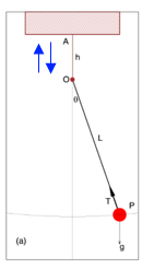
If we have a forced damped pendulum like this one:

Figure 1 – the blue arrows indicate that the point O is being driven up and down by an external force

-we also get a chaotic system.

What am I talking about? What is linear & non-linear? What is a “chaotic system”?

Digression on Non-Linearity for Non-Technical People

Common experience teaches us about linearity. If I pick up an apple in the supermarket it weighs about 0.15 kg or 150 grams (also known in some countries as “about 5 ounces”). If I take 10 apples the collection weighs 1.5 kg. That’s pretty simple stuff. Most of our real world experience follows this linearity and so we expect it.

On the other hand, if I was near a very cold black surface held at 170K (-103ºC) and measured the radiation emitted it would be 47 W/m². Then we double the temperature of this surface to 340K (67ºC) what would I measure? 94 W/m²? Seems reasonable – double the absolute temperature and get double the radiation.. But it’s not correct.

The right answer is 758 W/m², which is 16x the amount. Surprising, but most actual physics, engineering and chemistry is like this. Double a quantity and you don’t get double the result.

It gets more confusing when we consider the interaction of other variables.

Let’s take riding a bike [updated thanks to Pekka]. Once you get above a certain speed most of the resistance comes from the wind so we will focus on that. Typically the wind resistance increases as the square of the speed. So if you double your speed you get four times the wind resistance. Work done = force x distance moved, so with no head wind power input has to go up as the cube of speed (note 4). This means you have to put in 8x the effort to get 2x the speed.

On Sunday you go for a ride and the wind speed is zero. You get to 25 km/hr (16 miles/hr) by putting a bit of effort in – let’s say you are producing 150W of power (I have no idea what the right amount is). You want your new speedo to register 50 km/hr – so you have to produce 1,200W.

On Monday you go for a ride and the wind speed is 20 km/hr into your face. Probably should have taken the day off.. Now with 150W you get to only 14 km/hr, it takes almost 500W to get to your basic 25 km/hr, and to get to 50 km/hr it takes almost 2,400W. No chance of getting to that speed!

On Tuesday you go for a ride and the wind speed is the same so you go in the opposite direction and take the train home. Now with only 6W you get to go 25 km/hr, to get to 50km/hr you only need to pump out 430W.

In mathematical terms it’s quite simple: F = k(v-w)², Force = (a constant, k) x (road speed – wind speed) squared. Power, P = Fv = kv(v-w)². But notice that the effect of the “other variable”, the wind speed, has really complicated things.

To double your speed on the first day you had to produce eight times the power. To double your speed the second day you had to produce almost five times the power. To double your speed the third day you had to produce just over 70 times the power. All with the same physics.

The real problem with nonlinearity isn’t the problem of keeping track of these kind of numbers. You get used to the fact that real science – real world relationships – has these kind of factors and you come to expect them. And you have an equation that makes calculating them easy. And you have computers to do the work.

No, the real problem with non-linearity (the real world) is that many of these equations link together and solving them is very difficult and often only possible using “numerical methods”.

It is also the reason why something like climate feedback is very difficult to measure. Imagine measuring the change in power required to double speed on the Monday. It’s almost 5x, so you might think the relationship is something like the square of speed. On Tuesday it’s about 70 times, so you would come up with a completely different relationship. In this simple case know that wind speed is a factor, we can measure it, and so we can “factor it out” when we do the calculation. But in a more complicated system, if you don’t know the “confounding variables”, or the relationships, what are you measuring? We will return to this question later.

When you start out doing maths, physics, engineering.. you do “linear equations”. These teach you how to use the tools of the trade. You solve equations. You rearrange relationships using equations and mathematical tricks, and these rearranged equations give you insight into how things work. It’s amazing. But then you move to “nonlinear” equations, aka the real world, which turns out to be mostly insoluble. So nonlinear isn’t something special, it’s normal. Linear is special. You don’t usually get it.

..End of digression

Back to Pendulums

Let’s take a closer look at a forced damped pendulum. Damped, in physics terms, just means there is something opposing the movement. We have friction from the air and so over time the pendulum slows down and stops. That’s pretty simple. And not chaotic. And not interesting.

So we need something to keep it moving. We drive the pivot point at the top up and down and now we have a forced damped pendulum. The equation that results (note 1) has the massive number of three variables – position, speed and now time to keep track of the driving up and down of the pivot point. Three variables seems to be the minimum to create a chaotic system (note 2).

As we increase the ratio of the forcing amplitude to the length of the pendulum (β in note 1) we can move through three distinct types of response:

simple response
a “chaotic start” followed by a deterministic oscillation
a chaotic system

This is typical of chaotic systems – certain parameter values or combinations of parameters can move the system between quite different states.

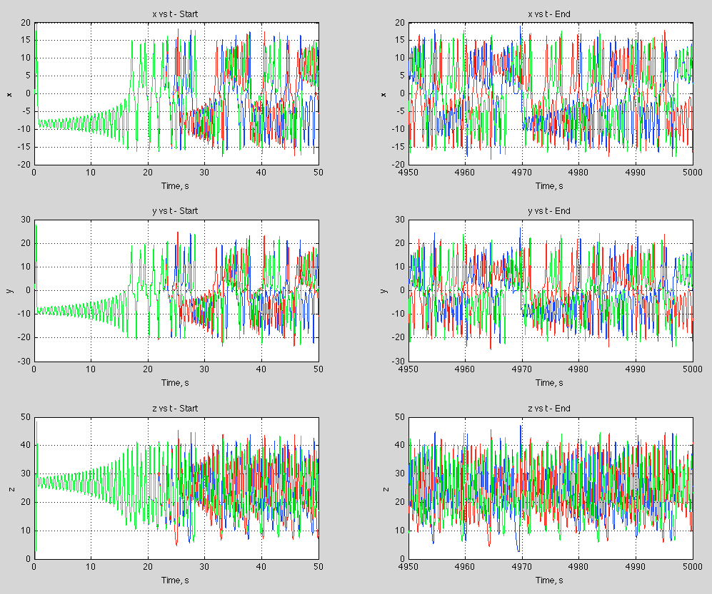
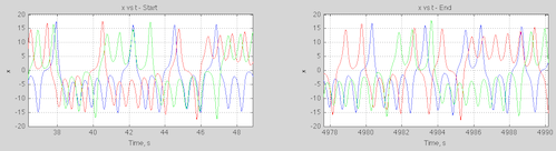
Here is a plot (note 3) of position vs time for the chaotic system, β=0.7, with two initial conditions, only different from each other by 0.1%:

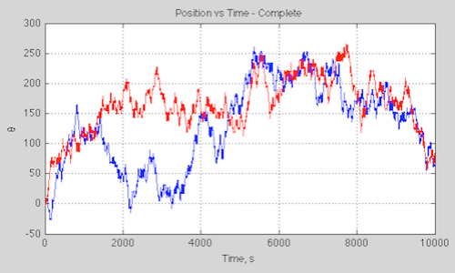
Forced damped harmonic pendulum, b=0.7: Start angular speed 0.1; 0.1001

Figure 1

It’s a little misleading to view the angle like this because it is in radians and so needs to be mapped between 0-2π (but then we get a discontinuity on a graph that doesn’t match the real world). We can map the graph onto a cylinder plot but it’s a mess of reds and blues.

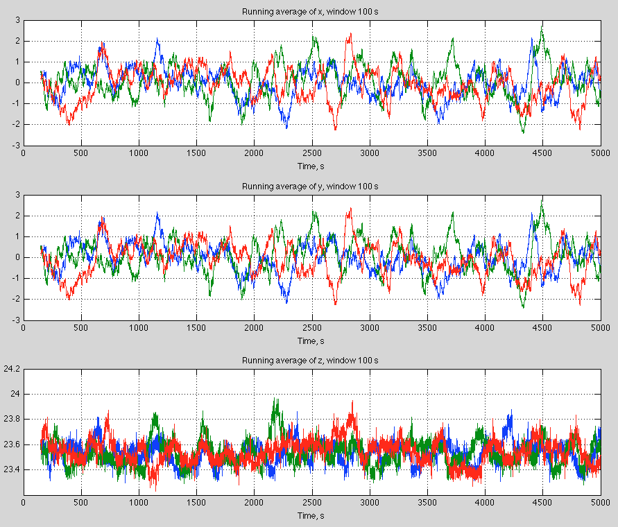
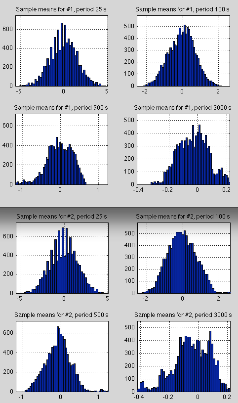
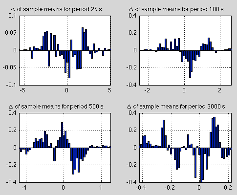
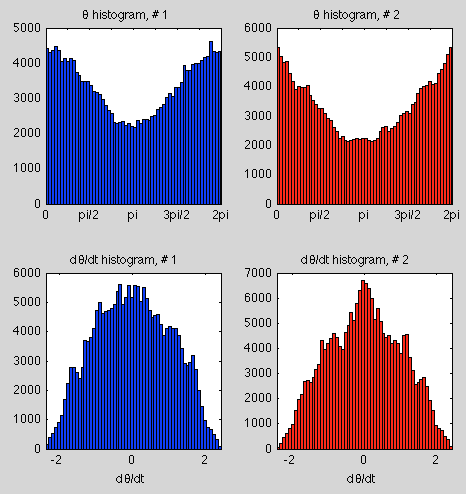
Another way of looking at the data is via the statistics – so here is a histogram of the position (θ), mapped to 0-2π, and angular speed (dθ/dt) for the two starting conditions over the first 10,000 seconds:

Histograms for 10,000 seconds

Figure 2

We can see they are similar but not identical (note the different scales on the y-axis).

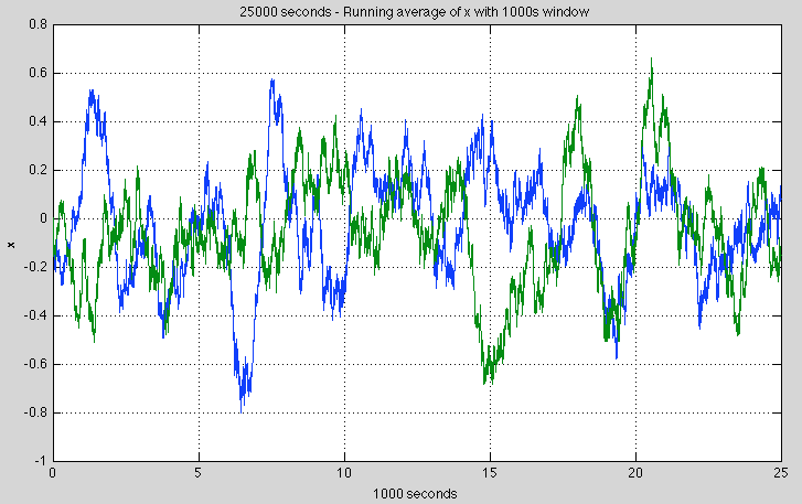
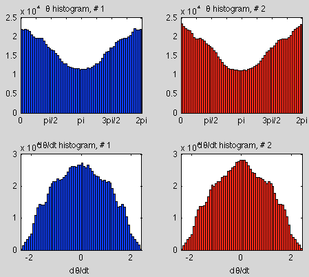
That might be due to the shortness of the run, so here are the results over 100,000 seconds:

Pendulum-0.7-100k seconds-2 conditions-hist

Histogram for 100,000 seconds

Figure 3

As we increase the timespan of the simulation the statistics of two slightly different initial conditions become more alike.

So if we want to know the state of a chaotic system at some point in the future, very small changes in the initial conditions will amplify over time, making the result unknowable – or no different from picking the state from a random time in the future. But if we look at the statistics of the results we might find that they are very predictable. This is typical of many (but not all) chaotic systems.

Orbits of the Planets

The orbits of the planets in the solar system are chaotic. In fact, even 3-body systems moving under gravitational attraction have chaotic behavior. So how did we land a man on the moon? This raises the interesting questions of timescales and amount of variation. Planetary movement – for our purposes – is extremely predictable over a few million years. But over 10s of millions of years we might have trouble predicting exactly the shape of the earth’s orbit – eccentricity, time of closest approach to the sun, obliquity.

However, it seems that even over a much longer time period the planets will still continue in their orbits – they won’t crash into the sun or escape the solar system. So here we see another important aspect of some chaotic systems – the “chaotic region” can be quite restricted. So chaos doesn’t mean unbounded.

According to Cencini, Cecconi & Vulpiani (2010):

Therefore, in principle, the Solar system can be chaotic, but not necessarily this implies events such as collisions or escaping planets..

However, there is evidence that the Solar system is “astronomically” stable, in the sense that the 8 largest planets seem to remain bound to the Sun in low eccentricity and low inclination orbits for time of the order of a billion years. In this respect, chaos mostly manifest in the irregular behavior of the eccentricity and inclination of the less massive planets, Mercury and Mars. Such variations are not large enough to provoke catastrophic events before extremely large time. For instance, recent numerical investigations show that for catastrophic events, such as “collisions” between Mercury and Venus or Mercury failure into the Sun, we should wait at least a billion years.

And bad luck, Pluto.

Deterministic, non-Chaotic, Systems with Uncertainty

Just to round out the picture a little, even if a system is not chaotic and is deterministic we might lack sufficient knowledge to be able to make useful predictions. If you take a look at figure 3 in Ensemble Forecasting you can see that with some uncertainty of the initial velocity and a key parameter the resulting velocity of an extremely simple system has quite a large uncertainty associated with it.

This case is quantitively different of course. By obtaining more accurate values of the starting conditions and the key parameters we can reduce our uncertainty. Small disturbances don’t grow over time to the point where our calculation of a future condition might as well just be selected from a randomly time in the future.

Transitive, Intransitive and “Almost Intransitive” Systems

Many chaotic systems have deterministic statistics. So we don’t know the future state beyond a certain time. But we do know that a particular position, or other “state” of the system, will be between a given range for x% of the time, taken over a “long enough” timescale. These are transitive systems.

Other chaotic systems can be intransitive. That is, for a very slight change in initial conditions we can have a different set of long term statistics. So the system has no “statistical” predictability. Lorenz 1968 gives a good example.

Lorenz introduces the concept of almost intransitive systems. This is where, strictly speaking, the statistics over infinite time are independent of the initial conditions, but the statistics over “long time periods” are dependent on the initial conditions. And so he also looks at the interesting case (Lorenz 1990) of moving between states of the system (seasons), where we can think of the precise starting conditions each time we move into a new season moving us into a different set of long term statistics. I find it hard to explain this clearly in one paragraph, but Lorenz’s papers are very readable.

Conclusion?

This is just a brief look at some of the basic ideas.

Articles in the Series

Natural Variability and Chaos – One – Introduction

Natural Variability and Chaos – Two – Lorenz 1963

Natural Variability and Chaos – Three – Attribution & Fingerprints

Natural Variability and Chaos – Four – The Thirty Year Myth

Natural Variability and Chaos – Five – Why Should Observations match Models?

Natural Variability and Chaos – Six – El Nino

Natural Variability and Chaos – Seven – Attribution & Fingerprints Or Shadows?

Natural Variability and Chaos – Eight – Abrupt Change

References

Chaos: From Simple Models to Complex Systems, Cencini, Cecconi & Vulpiani, Series on Advances in Statistical Mechanics – Vol. 17 (2010)

Climatic Determinism, Edward Lorenz (1968) – free paper

Can chaos and intransivity lead to interannual variation, Edward Lorenz, Tellus (1990) – free paper

Notes

Note 1 – The equation is easiest to “manage” after the original parameters are transformed so that tω->t. That is, the period of external driving, T0=2π under the transformed time base.

Then:

where θ = angle, γ’ = γ/ω, α = g/Lω², β =h0/L;

these parameters based on γ = viscous drag coefficient, ω = angular speed of driving, g = acceleration due to gravity = 9.8m/s², L = length of pendulum, h0=amplitude of driving of pivot point

Note 2 – This is true for continuous systems. Discrete systems can be chaotic with less parameters

Note 3 – The results were calculated numerically using Matlab’s ODE (ordinary differential equation) solver, ode45.

Note 4 – Force = k(v-w)² where k is a constant, v=velocity, w=wind speed. Work done = Force x distance moved so Power, P = Force x velocity.

Therefore:

P = kv(v-w)²

If we know k, v & w we can find P. If we have P, k & w and want to find v it is a cubic equation that needs solving.

Read Full Post »

Does the surface temperature change with “back radiation”? Kramm vs Gerlich

Posted in Basic Science, Commentary, Debunking Flawed "Science" on July 20, 2014| 113 Comments »

In The “Greenhouse” Effect Explained in Simple Terms I list, and briefly explain, the main items that create the “greenhouse” effect. I also explain why more CO2 (and other GHGs) will, all other things remaining equal, increase the surface temperature. I recommend that article as the place to go for the straightforward explanation of the “greenhouse” effect. It also highlights that the radiative balance higher up in the troposphere is the most important component of the “greenhouse” effect.

However, someone recently commented on my first Kramm & Dlugi article and said I was “plainly wrong”. Kramm & Dlugi were in complete agreement with Gerlich and Tscheuschner because they both claim the “purported greenhouse effect simply doesn’t exist in the real world”.

If it’s just about flying a flag or wearing a football jersey then I couldn’t agree more. However, science does rely on tedious detail and “facts” rather than football jerseys. As I pointed out in New Theory Proves AGW Wrong! two contradictory theories don’t add up to two theories making the same case..

In the case of the first Kramm & Dlugi article I highlighted one point only. It wasn’t their main point. It wasn’t their minor point. They weren’t even making a point of it at all.

Many people believe the “greenhouse” effect violates the second law of thermodynamics, these are herein called “the illuminati”.

Kramm & Dlugi’s equation demonstrates that the illuminati are wrong. I thought this was worth pointing out.

The “illuminati” don’t understand entropy, can’t provide an equation for entropy, or even demonstrate the flaw in the simplest example of why the greenhouse effect is not in violation of the second law of thermodynamics. Therefore, it is necessary to highlight the (published) disagreement between celebrated champions of the illuminati – even if their demonstration of the disagreement was unintentional.

Let’s take a look.

Here is the one of the most popular G&T graphics in the blogosphere:

From Gerlich & Tscheuschner

Figure 1

It’s difficult to know how to criticize an imaginary diagram. We could, for example, point out that it is imaginary. But that would be picky.

We could say that no one draws this diagram in atmospheric physics. That should be sufficient. But as so many of the illuminati have learnt their application of the second law of thermodynamics to the atmosphere from this fictitious diagram I feel the need to press forward a little.

Here is an extract from a widely-used undergraduate textbook on heat transfer, with a little annotation (red & blue):

From “Fundamentals of Heat and Mass Transfer” by Incropera & DeWitt (2007)

Figure 2

This is the actual textbook, before the Gerlich manoeuvre as I would like to describe it. We can see in the diagram and in the text that radiation travels both ways and there is a net transfer which is from the hotter to the colder. The term “net” is not really capable of being confused. It means one minus the other, “x-y”. Not “x”. (For extracts from six heat transfer textbooks and their equations read Amazing Things we Find in Textbooks – The Real Second Law of Thermodynamics).

Now let’s apply the Gerlich manoeuvre (compare fig. 2):

Fundamentals-of-heat-and-mass-transfer-post-G&T

Not from “Fundamentals of Heat and Mass Transfer”, or from any textbook ever

Figure 3

So hopefully that’s clear. Proof by parody. This is “now” a perpetual motion machine and so heat transfer textbooks are wrong. All of them. Somehow.

Just for comparison, we can review the globally annually averaged values of energy transfer in the atmosphere, including radiation, from Kiehl & Trenberth (I use the 1997 version because it is so familiar even though values were updated more recently):

From Kiehl & Trenberth (1997)

Figure 4

It should be clear that the radiation from the hotter surface is higher than the radiation from the colder atmosphere. If anyone wants this explained, please ask.

I could apply the Gerlich manoeuvre to this diagram but they’ve already done that in their paper (as shown above in figure 1).

So lastly, we return to Kramm & Dlugi, and their “not even tiny point”, which nevertheless makes a useful point. They don’t provide a diagram, they provide an equation for energy balance at the surface – and I highlight each term in the equation to assist the less mathematically inclined:

Figure 5

The equation says, the sum of all fluxes – at one point on the surface = 0. This is an application of the famous first law of thermodynamics, that is, energy cannot be created or destroyed.

The red term – absorbed atmospheric radiation – is the radiation from the colder atmosphere absorbed by the hotter surface. This is also known as “DLR” or “downward longwave radiation, and as “back-radiation”.

Now, let’s assume that the atmospheric radiation increases in intensity over a small period. What happens?

The only way this equation can continue to be true is for one or more of the last 4 terms to increase.

The emitted surface radiation – can only increase if the surface temperature increases
The latent heat transfer – can only increase if there is an increase in wind speed or in the humidity differential between the surface and the atmosphere just above
The sensible heat transfer – can only increase if there is an increase in wind speed or in the temperature differential between the surface and the atmosphere just above
The heat transfer into the ground – can only increase if the surface temperature increases or the temperature below ground spontaneously cools

So, when atmospheric radiation increases the surface temperature must increase (or amazingly the humidity differential spontaneously increases to balance, but without a surface temperature change). According to G&T and the illuminati this surface temperature increase is impossible. According to Kramm & Dlugi, this is inevitable.

I would love it for Gerlich or Tscheuschner to show up and confirm (or deny?):

yes the atmosphere does emit thermal radiation
yes the surface of the earth does absorb atmospheric thermal radiation
yes this energy does not disappear (1st law of thermodynamics)
yes this energy must increase the temperature of the earth’s surface above what it would be if this radiation did not exist (1st law of thermodynamics)

Or even, which one of the above is wrong. That would be outstanding.

Of course, I know they won’t do that – even though I’m certain they believe all of the above points. (Likewise, Kramm & Dlugi won’t answer the question I have posed of them).

Well, we all know why

Hopefully, the illuminati can contact Kramm & Dlugi and explain to them where they went wrong. I have my doubts that any of the illuminati have grasped the first law of thermodynamics or the equation for temperature change and heat capacity, but who could say.

Read Full Post »

“Blah blah blah” vs Equations

Posted in Basic Science, Commentary on January 30, 2012| 455 Comments »

It is not surprising that the people most confused about basic physics are the ones who can’t write down an equation for their idea.

The same people are the most passionate defenders of their beliefs and I have no doubts about their sincerity.

I’ll meander into what it is I want to explain..

I found an amazing resource recently – iTunes U short for iTunes University. Now I confess that I have been a little confused about angular momentum. I always knew what it was, but in the small discussion that followed The Coriolis Effect and Geostrophic Motion I found myself wondering whether conservation of angular momentum was something independent of, or a consequence of, linear momentum or some aspect of Newton’s laws of motion.

It seemed as if conservation of angular momentum was an orphan of Newton’s three laws of motion. How could that be? Perhaps this conservation is just another expression of these laws in a way that I hadn’t appreciated? (Knowledgeable readers please explain).

Just around this time I found iTunes U and searched for “mechanics” and found the amazing series of lectures from MIT by Prof. Walter Lewin. A series of videos. I recommend them to anyone interested in learning some basics about forces, motion and energy. Lewin has a gift, along with an engaging style. It’s nice to see chalk boards and overhead projectors because they are probably no more in use (? young people please advise).

These lectures are not just for iPhone and iTunes people – here is the weblink.

The gift of teaching science is not in accuracy – that’s a given – the gift is in showing the principle via experiment and matching it with a theoretical derivation, and “why this should be so” and thereby producing a conceptual idea in the student.

I haven’t got to Lecture 20: Angular Momentum yet, I’m at about lecture 11. It’s basic stuff but so easy to forget (yes, quite a lot of it has been forgotten). Especially easy to forget how different principles link together and which principle is used to derive the next principle.

What caught my attention for the purposes of this article was how every principle had an equation.

For example, in deriving the work done on an object, Lewin integrates force over the distance traveled and comes up with the equation for kinetic energy.

While investigating the oscillation of a mass on a spring, the equation for its harmonic motion is derived.

Every principle has an equation that can be written down.

Over the last few days, as at many times over the past two years, people have arrived on this blog to explain how radiation from the atmosphere can’t affect the surface temperature because of blah blah blah. Where blah blah blah sounds like it might be some kind of physics but is never accompanied by an equation.

Here’s the equation I find in textbooks.

Energy absorbed from the atmosphere by the surface, E_a:

E_a = αR_L↓ ….[eqn 1]

where α = absorptivity of the surface at these wavelengths, R_L↓ = downward radiation from the atmosphere

And this energy absorbed, once absorbed, is indistinguishable from the energy absorbed from the sun. 1 W/m² absorbed from the atmosphere is identical to 1 W/m² absorbed from the sun.

That’s my equation. I have provided six textbooks to explain this idea in a slightly different way in Amazing Things we Find in Textbooks – The Real Second Law of Thermodynamics.

It’s also produced by Kramm & Dlugi, who think the greenhouse effect is some unproven idea:

Now the equation shown is a pretty simple equation. The equation reproduced in the graphic above from Kramm & Dlugi looks a little more daunting but is simply adding up a number of fluxes at the surface.

Here’s what it says:

Solar radiation absorbed + longwave radiation absorbed – thermal radiation emitted – latent heat emitted – sensible heat emitted + geothermal energy supplied = 0

Or another way of thinking about it is energy in = energy out (written as “energy in – energy out = 0“)

Now one thing is not amazing to me – of the tens (hundreds?) of concerned citizens commenting on the many articles on this subject who have tried to point out my “basic mistake” and tell me that the atmosphere can’t blah blah blah, not a single one has produced an equation.

The equation might look something like this:

E_a = f(α,T_atm-T_sur).R_L↓ ….[eqn 2]
where T_atm = temperature of the atmosphere, T_sur = temperature of the surface

With the function f being defined like this:

f(α,T_atm-T_sur) = α, when T_atm ≥ T_sur and

f(α,T_atm-T_sur) = 0, when T_atm < T_sur

In English, it says something like energy from the atmosphere absorbed by the surface = 0 when the temperature of the atmosphere is less than the temperature of the surface.

I’m filling in the blanks here. No one has written down such ridiculous unphysical nonsense because it would look like ridiculous unphysical nonsense. Or perhaps I’m being unkind. Another possibility is that no one has written down such ridiculous unphysical nonsense because the proponents have no idea what an equation is, or how one can be constructed.

My Prediction

No one will produce an equation which shows how no atmospheric energy can be absorbed by the surface. Or how atmospheric energy absorbed cannot affect internal energy.

This is because my next questions will be:

Please supply a textbook or paper with this equation
Please explain from fundamental physics how this can take place

My Challenge

Here’s my challenge to the many people concerned about the “dangerous nonsense” of the atmospheric radiation affecting surface temperature –

Supply an equation.

If you can’t, it is because you don’t understand the subject.

It won’t stop you talking, but everyone who is wondering and reads this article will be able to join the dots together.

The Usual Caveat

If there were only two bodies – the warmer earth and the colder atmosphere (no sun available) – then of course the earth’s temperature would decrease towards that of the atmosphere and the atmosphere’s temperature would increase towards that of the earth until both were at the same temperature – somewhere between the two starting temperatures.

However, the sun does actually exist and the question is simply whether the presence of the (colder) atmosphere affects the surface temperature compared with if no atmosphere existed. It is The Three Body Problem.

My Second Prediction

The people not supplying the equation, the passionate believers in blah blah blah, will not explain why an equation is not necessary or not available. Instead, continue to blah blah blah.

Read Full Post »

« Newer Posts - Older Posts »

	DeWitt Payne on CO2 – An Insignificant T…
	Jay Coalson on CO2 – An Insignificant T…
	Frank on Clouds and Water Vapor –…
	Frank on Clouds and Water Vapor –…
	nobodysknowledge on Clouds and Water Vapor –…
	DeWitt Payne on Models, On – and Off…
	Frank on Models, On – and Off…
	Hugo Kramer on CO2 Can’t have that Effe…
	DeWitt Payne on Clouds and Water Vapor –…
	nobodysknowledge on Clouds and Water Vapor –…
	nobodysknowledge on Clouds and Water Vapor –…
	Frank on Renewables XIV – Minimiz…
	nobodyknowledge on Clouds and Water Vapor –…
	DeWitt Payne on Renewables XIV – Minimiz…
	scienceofdoom on Renewables XIV – Minimiz…

Evaluating and Explaining Climate Science

Archive for the ‘Commentary’ Category

Climate Models

Crop Models

Economic Models

Conclusion

References

Notes

Articles in this Series

References

Calculating the Cost

Moore’s Law and Other Industries

Intermittency & Grid Operators

The Other Side of the Equation – Conventional Power

$ and GHG emissions

Conclusion – Introduction

Articles in this Series

References

Step 1 – The ‘greenhouse’ effect

Step 2 – AGW = ‘Greenhouse effect’ plus feedbacks

Step 3 – Attribution Studies

Step 4 – Unprecedented Temperature Rises

Conclusion

Attractors and Phase Space

Conclusion

Articles in the Series

References

Notes

Pendulums

Digression on Non-Linearity for Non-Technical People

Back to Pendulums

Orbits of the Planets

Deterministic, non-Chaotic, Systems with Uncertainty

Transitive, Intransitive and “Almost Intransitive” Systems

Conclusion?

Articles in the Series

References

Notes

My Prediction

My Challenge

The Usual Caveat

My Second Prediction

Pages

Recent Posts

Recent Comments

Categories

Climate Websites

Science of Doom Key Pages

Subscribe by RSS

Subscribe by Email

Archives

Meta